Building an Ultra-High Throughput AI-SQL Engine
1. AI-SQL makes unstructured data useful, but it is expensive.
Fast LLM classifiers have been taking over the internet lately. Jev is the clearest example: give a model a small, bounded decision and get an answer almost immediately. What better place to run millions of those decisions than… inside the database!
Indeed, database vendors have recently begun to offer this kind of intelligence at scale through AI-SQL, also called AI functions. AI-SQL extends SQL with user-defined functions that invoke LLMs. Users specify each function with a natural-language prompt. A query can look like this:
SELECT *
FROM reviews AS r
WHERE AI.IF(PROMPT('Does this review discuss the ending?\n\n{0}', r.review));
Many database vendors support AI-SQL. For example, Snowflake Cortex AISQL, BigQuery AI functions, Databricks AI Functions, and, recently, MotherDuck all support it.
Unfortunately, executing AI-SQL is extremely expensive. An AI function evaluates its prompt row by row, so one SQL query can create hundreds of thousands or millions of model calls. A filter needs one LLM call per row. A naive join needs one LLM call for every pair of rows in its two input tables.
This line of work has become extremely popular in the database research community. A number of open-source academic systems have emerged, including our work on DocETL from UC Berkeley, LOTUS from Stanford, Palimpzest from MIT, and ThalamusDB from Cornell. These systems (and database vendors) primarily reduce cost by eliminating as many LLM calls as possible (e.g., MOAR, Task Cascades, and Abacus) and by using cheaper models when possible (e.g., BARGAIN). Even after these optimizations, a query plan may still require hundreds of thousands or millions of LLM calls.
2. Key Idea: Query plans should control LLM inference!
A natural thought is to use a general-purpose inference engine such as vLLM to execute the query plan. However, sending millions of related model calls to vLLM as separate requests has a large cost! We’ll illustrate with the following query:
Given a dataset of medical reports and a dataset of possible adverse reactions, find serious adverse event reports that mention both a cardiovascular reaction and a neurological reaction.1
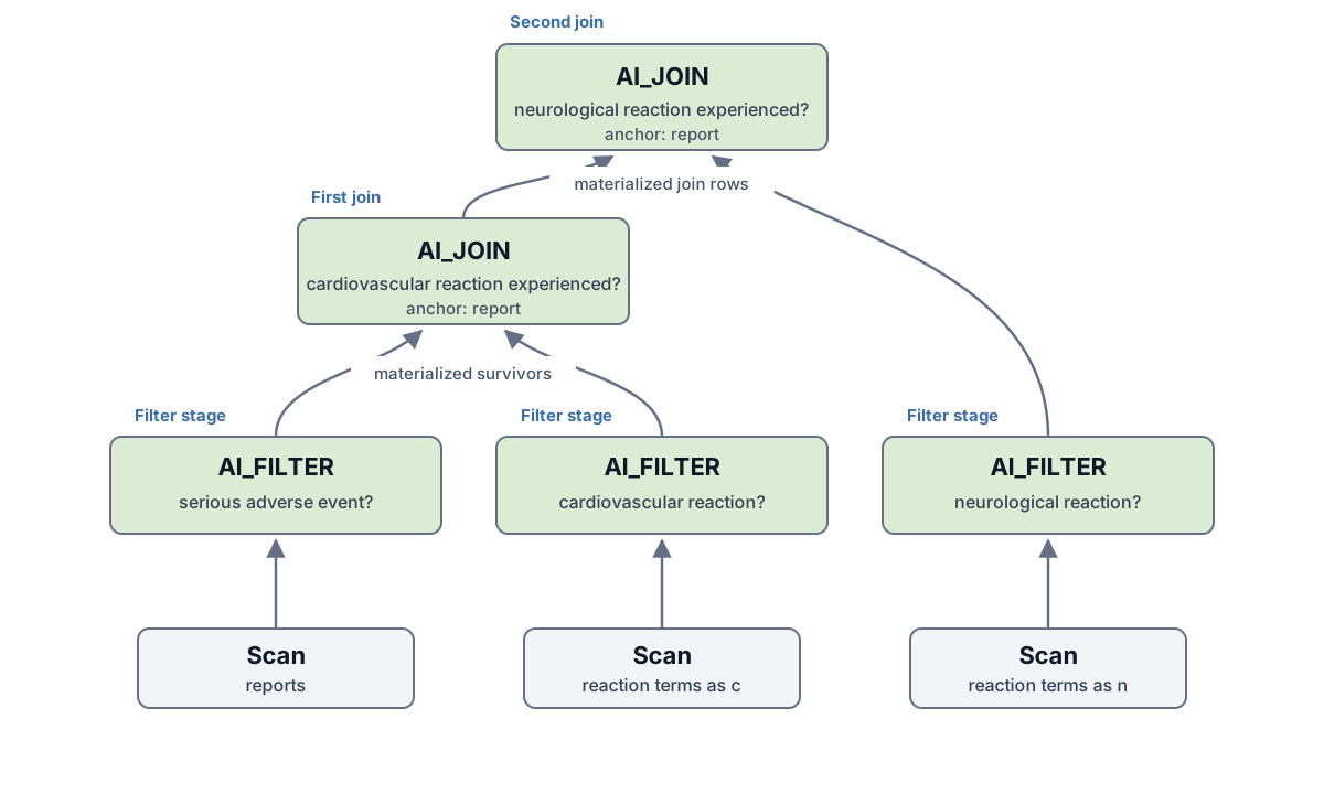
We call this query BIO-4 in QUAIL-B, a benchmark we are building to evaluate AI-SQL query engines. Its inputs contain 5,000 long reports and 4,144 reaction terms (the latter is used twice, as there are two joins). The logical plan, shown in Figure 1, works as follows:
-
It filters the reports for serious adverse events.
-
It filters the two reaction term dataset inputs (i.e., lists of possible adverse reaction terms) for cardiovascular and neurological reactions.
-
It joins the surviving reports with the cardiovascular terms, then with the neurological terms.
How might we execute BIO-4 with vLLM? Following what databases do, we’d render one prompt for each filter input, and, for the join, one prompt for candidate report and reaction pair. Each prompt would be a separate inference request.2 For the filters, there’s just one document per prompt; for the join, we’d place the much longer medical report first as the anchor and the reaction term second as the partner to maximize reuse of the prefix’s key and value state (KV) across join prompts. We’d execute one operator at a time and order its LLM requests so requests for the same document are evaluated together, maximizing KV reuse.
A cost estimate for the query plan. Before running the vLLM baseline, we first want to estimate the lowest possible runtime for the same plan. We count the model’s arithmetic work and HBM traffic from the token lengths, then use a roofline model to estimate the time. The estimate assumes peak GPU throughput, full overlap between CPU and GPU work, and unlimited space for retained KV. No implementation can meet all of these assumptions, so this optimistic lower bound is our speed of light estimate, or SoL. For BIO-4, the SoL estimate is 894.37 seconds, or 14.91 minutes.3 The implementation in Quail contains the full calculation (which we’ll discuss in a follow-up blog post).
How we hoped vLLM would perform. Each request produces one token constrained to TRUE or FALSE, so all model work is prefill. BIO-4 compiles to millions of requests, so there should always be a large batch ready for the H100. With a large enough batch, vLLM should keep the H100 busy, and get as close to the SoL estimate as possible.
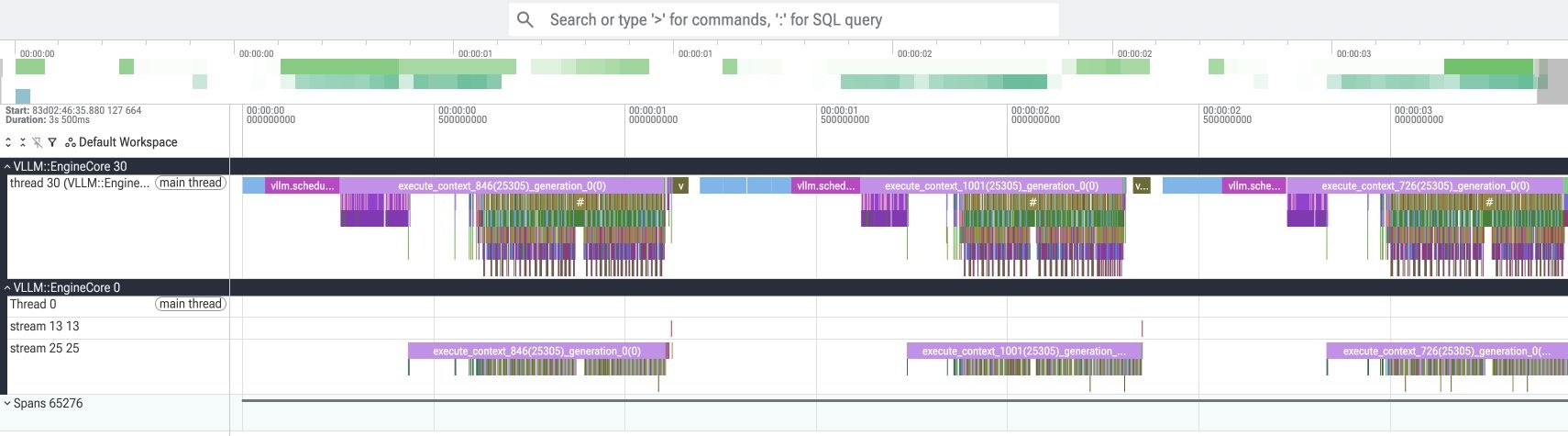
How vLLM actually performs. We run vLLM 0.26.0 with Qwen3 4B FP8 on one H100. We give it enough batch capacity to use the GPU. At scale factor 1.0, a vLLM baseline takes 6.84 hours, or 27.55x the SoL estimate! There are two reasons for the inefficiency. Figure 2 shows a representative 3.5-second window from the first join.
-
The primary reason is host overhead. The CPU spends long stretches scheduling and tracking requests while the H100 waits, as shown by the gaps in Figure 2.4
-
The second is KV regret: vLLM sometimes discards KV that it needs again later. On BIO-4 at scale factor 1.0, it therefore processes 174.6 million tokens instead of 124.3 million: 50.3 million extra tokens, or 40% more work.
We can, and we should, reduce both sources of waste by optimizing inference for AI-SQL!
3. We built Quail to run AI-SQL queries faster.
We will first show you how you can get started. To skip to read about how Quail works, skip to Section 3.2.
3.1 You can run your first Quail query in a few lines of code!This part is collapsible, for space reasons.
We can use Quail to run two AI filters over all 100,000 movie reviews in the Stanford IMDB dataset. We first download the reviews from Hugging Face, and load them into an Arrow dataset.
import pyarrow as pa
import pyarrow.dataset as ds
from datasets import concatenate_datasets, load_dataset
import quail

imdb = load_dataset(
    "stanfordnlp/imdb",
    revision="e6281661ce1c48d982bc483cf8a173c1bbeb5d31",
)
all_reviews = concatenate_datasets([
    imdb["train"],
    imdb["test"],
    imdb["unsupervised"],
])
reviews = ds.dataset(pa.table({
    "review_id": pa.array(f"review-{i}" for i in range(len(all_reviews))),
    "review": all_reviews.data.table.column("text"),
}))
The query keeps reviews that discuss the movie’s ending, and recommend watching the movie.
# This Python process has access to one H100.
config = quail.EngineConfig(
    gpus=1,
    model="qwen3-4b-fp8",
    backend="quail",
    device="h100-sxm",
)
with quail.Session(config) as session:
    session.register(
        "reviews",
        quail.DocumentProvider.from_dataset(reviews, id_col="review_id"),
    )

    query = session.sql("""
        SELECT r.review_id
        FROM reviews AS r
        WHERE AI.IF(
            PROMPT(
                'Does this review discuss the ending of the movie?\n\n{0}',
                r.review
            ),
            -- Optional, but helps Quail reorder filters.
            {'selectivity': 0.25}
        )
        AND AI.IF(
            PROMPT(
                'Does the reviewer recommend watching the movie?\n\n{0}',
                r.review
            ),
            {'selectivity': 0.5}
        )
    """, dialect="bq")

    print(query.explain())
    result = query.run()
    table = result.collect()
Before running the query, query.explain() prints the logical and physical plans. The output below keeps only the parts that describe the two filters and their execution settings.
logical:
Project: r.review_id
SemanticFilter
predicate 1: discusses the ending (selectivity=25%)
predicate 2: recommends the movie (selectivity=50%)
Scan reviews as r [review, review_id]

physical: backend=quail, model=qwen3-4b-fp8, workers=1
KV=bf16
chunk budget=110,376 tokens
admission budget=362,250 tokens
Project: r.review_id (est. rows=12,500)
AiFilter: r (est. rows=12,500; est. time=124 s)
KV rewind=on
predicate 1 (input rows=100,000; est. pass=25%)
predicate 2 (input rows=25,000; est. pass=50%)
Scan reviews as r (rows=100,000)
tokens=29,926,924, mean_doc_tokens=299.3
The complete example in demos/imdb_ending_filter.py prints the following results at the end of the run:
matching reviews: 16057 of 100000
stage evaluated 100000 reviews, 0.283 passed
stage evaluated 28296 reviews, 0.568 passed
boot_s: 57.65 (cold)
token_wait_s: 0.0
wall_s: 277.41
total_s: 335.06 (boot + query)
fresh_tokens: 32499738
documents/second: 360.5
GPU price: $3.9492/GPU-hour (Modal)
GPU cost, including startup: $0.3675
The full run costs $0.3675 at Modal’s H100 price, including model startup.5 At current GPT-5 nano prices (including cached token prices), the same two-filter workload would cost about $1.75, or 4.8 times the measured Quail cost!6
Running on Modal. If you don’t have a dedicated GPU, you can put the whole query inside a Modal GPU function. The function creates a normal Quail session and runs it:
import modal

app = modal.App("quail-engine")
image = (
    modal.Image.from_registry(
        "nvidia/cuda:13.0.1-devel-ubuntu24.04",
        add_python="3.12",
    )
    .entrypoint([])
    .uv_pip_install("quail-engine==0.1.0")
)

@app.function(image=image, gpu="H100!", memory=32768, timeout=1200)
def run_query(sql, documents):
    import quail

    config = quail.EngineConfig(
        gpus=1,
        model="qwen3-4b-fp8",
        backend="quail",
        device="h100-sxm",
    )
    with quail.Session(config) as session:
        session.register(
            "docs",
            quail.DocumentProvider.from_table(documents, id_col="id"),
        )
        result = session.sql(sql).run()
        return result.collect(), result.report
Modal allocates the H100, and Quail plans and runs the query inside the function. A complete example is in demos/quickstart_modal.py.
Check out the Quail documentation to learn more.
3.2 Quail jointly plans queries and inference.
This section describes Quail’s main design ideas at a high level. We are still actively building Quail, and we will provide the full technical details in a future report.
We have three performance goals for Quail:
-
Minimize KV regret.
-
Keep the GPU busy by reducing CPU scheduling overhead.
-
Reach high model FLOP/s utilization (MFU) while the GPU is active.
Our current evaluation focuses on the first two goals. We defer a full MFU study to future work.
As shown in Figure 3, Quail consists of a query frontend, a query planner, and an execution engine. Through the frontend, the user provides Arrow tables or datasets, an AI-SQL or Python query, and the model and GPU or GPUs to use. The frontend creates a logical plan from the query. The query planner orders the filters and joins, chooses the anchor for each join, and determines how many tokens each model forward pass should process. The planner then lowers the logical plan into a physical operator plan, which the execution engine runs.
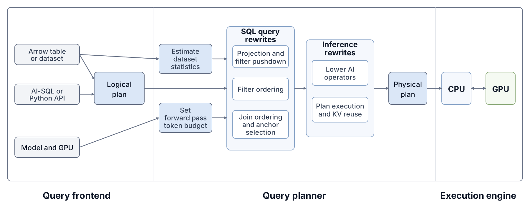
Quail is extensible, and its design is inspired by Apache DataFusion, an open source, extensible analytical query engine. One can add new query operators, planning rules, execution backends, models, or support for other hardware.
3.2.1 Quail turns AI-SQL into a logical query plan.
Users register data as an in-memory Arrow table or an Arrow dataset. Users can write queries in AI-SQL (we support both Snowflake’s and BigQuery’s spellings, AI_FILTER and AI.IF), or use a Python query builder similar to pandas. The current release of Quail supports AI filters and joins, along with relational projections and LIMIT.
Users define each AI operator with a prompt and can provide optional planning information. The optional selectivity gives the expected fraction of documents or document pairs that will pass; without it, Quail keeps predicates in their written order. For a join, the optional anchor chooses which input comes first in the prompt for KV reuse; without it, the planner chooses the anchor.
Users can specify the model and GPU count. Quail currently supports three models: Qwen3 4B FP8, Qwen3 32B FP8, and DiffusionGemma on H100 GPUs. We plan to add support for more models and hardware through the extension interface.
In Quail, each AI-SQL query is parsed with SQLGlot into a logical plan, which is then passed to the query planner.
3.2.2 Quail plans operator order and KV reuse.
Database query optimizers already use many rules, e.g., pushing down filters, reordering predicates, and choosing join order. AI-SQL adds several new decisions, e.g., which document should be the join anchor, which KV will be needed by a later operator, and how much model work should enter each forward pass. Quail plans both kinds of decisions together.
Overview. Given the logical query plan, we do the following:
-
Compute dataset statistics. We estimate the document lengths and basic statistics for each input dataset.
-
Compute forward pass and KV limits. From the selected model and GPU, we choose how many tokens to process in each model forward pass and calculate the fixed KV capacity.
-
Perform SQL query rewrites. We push down projections and filters, order the filters, and choose the join order and anchor for each join.
-
Perform Inference-specific query rewrites. We lower AI operations into physical operators and plan their execution order and KV use.
We describe these steps at a high level, in turn.
Dataset statistics. We estimate the row count, average document length, and maximum document length for each input dataset.
Forward pass and KV limits. Given the user’s selected model size and GPU memory size, we calculate the maximum number of tokens to compute for each model forward pass. We reserve HBM for the model weights and two forward passes, and leave the rest of the HBM for the KV cache. (This is more conservative than vLLM, which profiles one forward pass to determine how much activation memory to reserve, so we can probably improve on this).
SQL query rewrites. We push projections and filters down to the source datasets. We order filters using their estimated cost and selectivity, following extremely well-known prior work (Hellerstein and Stonebraker et al.). For joins, we use a Selinger-style search (i.e., System R) to choose the join order and anchor for each join. The cost model uses the speed-of-light estimate from Section 2. We will explain the calculation in a future post. For now, you can check out the cost model code.
Inference-specific query rewrites. After the SQL rewrites, we translate the logical plan into a DAG of physical operators. You can find the physical operators that Quail currently supports in our physical plan documentation. For example, the AiFilter physical operator evaluates AI predicates over documents, while AiJoin evaluates AI predicates over document pairs that share an anchor. Each AI physical operator also specifies its prompt, model, forward pass token budget, and KV settings (e.g., whether to write KV to HBM because there will be a subsequent operator in the query).
Drawing inspiration from vectorized query execution, Quail streams intermediate results directly between operators rather than materializing complete datasets on disk or in main memory. For example, in BIO-4, as soon as a batch of reports passes the initial filter operator, Quail immediately pipelines it to the first join operator. It maintains the report KV cache in HBM throughout both join operations, allowing direct comparisons against the filtered reaction terms without redundant KV recomputations.
3.2.3 Quail runs the physical query plan.
Overview. The execution engine has three main components:
-
Physical plan executor. On the CPU, Quail pulls document batches through the physical operator DAG and prepares work for the GPU.
-
KV manager. Quail allocates, pins, “rewinds” (i.e., only persists KV for the prefix we know will appear in a future operator, not the entire LLM prompt which includes the document(s) and some natural language instruction), and releases KV pages according to the physical plan.
-
Inference program. On the GPU, Quail runs a model forward pass for each input batch.
Figure 4 shows how these components work together.
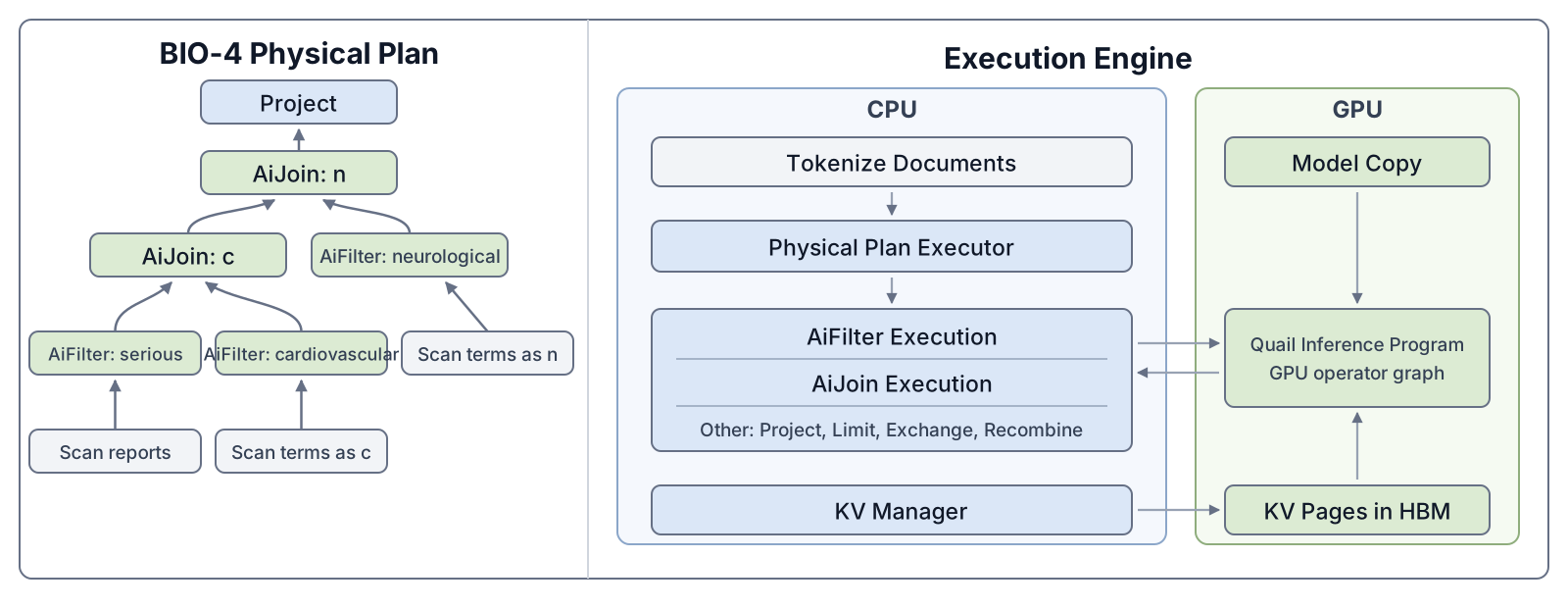
We’ll discuss the first two components; then we’ll describe the inference program in Section 3.2.4.
Physical plan executor. Quail uses a pull-based executor, as in Volcano, but processes a batch at a time, as in MonetDB. Before execution, Quail tokenizes every document column referenced by an AI filter or join with Gigatoken7, then loads one model copy per GPU. During execution, the CPU prepares one input batch while the GPU processes another.
KV manager. Each GPU has a fixed pool of KV pages in HBM. After each model evaluation, Quail retains only the KV that a later evaluation can reuse. For a filter, Quail places the document before the predicate-specific question. After the predicate returns TRUE or FALSE, Quail discards the predicate KV and “rewinds” to the end of the document KV. Then, if the predicate returns TRUE and another AI operator uses the document, Quail will retain the “rewinded” KV in HBM; otherwise, Quail will release it. Quail similarly retains “rewinded” KV for joins. If eviction is necessary, Quail evicts the shortest documents, since longer documents take disproportionately longer to recompute, thanks to attention being a quadratic operation.
Note that a general-purpose inference is different in that: (1) it retains all the KV associated with a request (no “rewinding”), even though the suffix KV will never be used again in the query, (2) all requests’ KV are wastefully saved in HBM, even if documents are filtered out in the query and never needed again, and (3) documents are evicted with LRU.
Using multiple GPUs. Our current multi-GPU support is quite basic. We place one complete model copy and one KV pool on each GPU. We partition filter documents and join anchors randomly and uniformly across the GPUs, run them independently, and combine the results on the CPU.
3.2.4 Quail uses specialized inference programs for AI-SQL.
During planning, Quail chooses which documents or document pairs require model evaluation. During execution, each evaluation follows an inference program: e.g., embedding lookup, transformer layers, attention, matrix multiplication, etc.
Here, we first describe how physical operators are expressed as inference programs, then how vLLM represents an inference program (which we adopt), and finally, the changes we make to Quail’s inference program.
Physical operator interface. Each AiFilter or AiJoin physical operator is expressed as an inference program. The program takes token IDs and positions, plus the locations of any reusable KV pages. It returns TRUE and FALSE scores for each row or pair of rows. Quail runs the program across all rows or pairs evaluated by the operator.
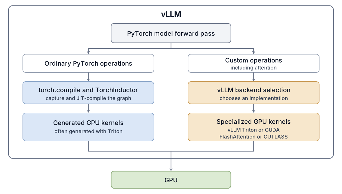
vLLM’s inference programs. vLLM is a general-purpose engine designed to support any inference pattern, across various model architectures and hardware backends. How does vLLM do it all? As shown in Figure 5, given the model choice and GPU, there are two primary paths through which vLLM creates an inference program (i.e., of GPU kernels): (1) PyTorch operations JIT-compiled with torch.compile and TorchInductor into generated Triton GPU kernels, and (2) custom operations (such as attention) expressed through highly specialized GPU kernels like, FlashAttention.
Quail’s inference program. We did not reimplement every model and GPU operation from scratch. That would be silly. Instead, Quail uses vLLM’s model implementations to obtain the operations required for a forward pass, then runs them with its own scheduler and KV manager. However, Quail makes three small changes to the forward pass:
First, fuse small operations. We write Triton kernels that fuse normalization with FP8 quantization, Q/K normalization with RoPE, and activation with FP8 quantization. This is extremely easy to do now with AI agents; it requires no novel kernel design ideas. By fusing these operations, Quail reduces kernel launches and intermediate HBM traffic.8
Second, specialize attention for joins. An AI join compares one anchor with many partners. Standard vLLM treats each anchor and partner as a separate sequence. Attention therefore reads the same anchor KV again for every partner, as the left side of Figure 6 shows.
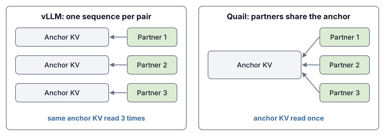
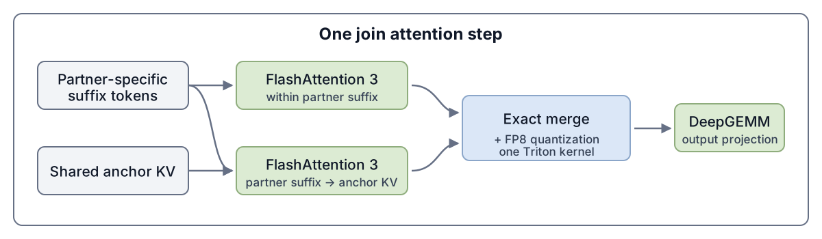
Quail groups all partners that share an anchor and computes the anchor KV once (right side of Figure 6). Figure 7 shows how Quail evaluates attention in two parts. One FlashAttention 3 call computes causal attention within each partner. A second call applies all partner queries to the shared anchor KV, reducing repeated reads. Quail combines the two results using their log-sum-exp values and the online softmax formula, producing the same output as attention over each full anchor and partner sequence. This is one level of “tree”-based attention.9 One Triton kernel combines the BF16 outputs and converts them to the FP8 format expected by the output projection.
Third, restrict the output head to TRUE and FALSE. Normally, a model would use its final output head (“language modeling” head, lm_head) to compute a score for every token in its vocabulary. For AI filters and joins, Quail needs only the scores for token IDs that represent TRUE or FALSE.10 Quail therefore multiplies the final hidden state by only the corresponding rows of the output/language modeling head matrix. By using the smaller matrix, Quail reduces computation and GPU memory use by the output head.
4. We evaluate Quail against vLLM.
At scale factor 0.1, Quail is faster than a “stock” vLLM baseline on 27 of the 29 QUAIL-B queries. The (geometric) mean speedup is 1.84x, and the maximum speedup is 11.22x on BIO-2. At scale factor 1.0, we find a query for which Quail is 14.04x faster! The two queries where stock vLLM wins expose one missing feature clearly: Quail does not yet reuse matching prefixes across different rows.
In this section, we first describe our metrics and baselines, then present the full QUAIL-B results, and finally examine BIO-4 and AGENT-1 in detail.
4.1 Metrics and baselines for AI-SQL performance.
Metrics. We report three metrics for each query: KV regret, $/query, and input tokens/second. KV regret is repeated model work: fresh input tokens beyond the minimum needed to compute each reusable prefix once. $/query is query runtime in hours multiplied by $3.9492 per H100-hour. Input tokens/second is the total requested input tokens divided by query runtime. Each evaluated prompt contributes its full input length, including tokens served from KV. Lower KV regret and cost are better; higher throughput is better.
QUAIL-B. We created QUAIL-B, a benchmark with 29 AI-SQL queries. It covers IMDB reviews, medical reports, fact-checking claims, legal documents, and software-agent traces. Queries include filters, filter sequences, and one or more joins. Each dataset has scale factors 0.1, 0.5, and 1.0. We compare all 29 default queries at scale factor 0.1. We examine BIO-4 at scale factor 1.0 and AGENT-1 in more detail.
Setup. Every query uses Qwen3 4B FP8 with BF16 KV on one H100. Quail and each vLLM baseline run one after the other on the same physical GPU. They use the same model, prompts, and logical query plan.
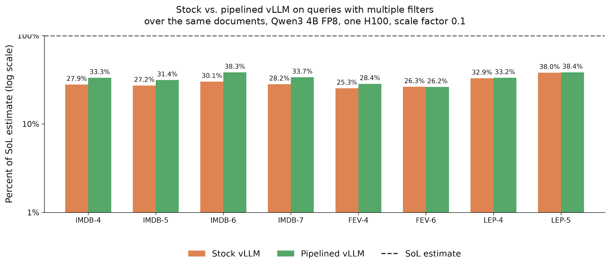
vLLM baselines. Both baselines use the optimal operator ordering chosen by our query planner. For each operator, we prepare its requests and order them to improve KV reuse. We call the operator-at-a-time baseline “stock vLLM.” For QUAIL-B queries with multiple filters or joins, we also report a “pipelined vLLM” baseline. It pipelines requests between consecutive filters and between consecutive joins. For fairness, both baselines use Gigatoken for tokenization, as Quail does, instead of vLLM’s Hugging Face tokenizer.11
4.2 Overall, Quail is 1.84x faster across QUAIL-B.
Table 1 averages tokens/second, KV regret, and cost per query within each dataset at scale factor 0.1. Cost multipliers are relative to Quail.
| Dataset | Quail | Stock vLLM |
|---|---|---|
| BIO (4 queries) | 12,296,410 tokens/s 157,995 KV regret $0.0892/query (1.00x) |
1,420,421 tokens/s 1,441,816 KV regret $0.7771/query (8.72x) |
| IMDB (10 queries) | 649,864 tokens/s 451,917 KV regret $0.0282/query (1.00x) |
382,818 tokens/s 1,129,174 KV regret $0.0467/query (1.66x) |
| FEV (8 queries) | 1,692,276 tokens/s 408,592 KV regret $0.0383/query (1.00x) |
724,574 tokens/s 519,588 KV regret $0.0820/query (2.14x) |
| LEP (5 queries) | 388,903 tokens/s 2,147 KV regret $0.0670/query (1.00x) |
316,617 tokens/s 70,982 KV regret $0.0853/query (1.27x) |
| AGENT (2 queries) | 73,006 tokens/s 11,886,152 KV regret $0.2616/query (1.00x) |
169,201 tokens/s 23,928 KV regret $0.1129/query (0.43x) |
Table 1. Average QUAIL-B results by dataset at scale factor 0.1. Cost multipliers are relative to Quail.
Figure 8 summarizes throughput by dataset, and Figure 9 reports latency for all 29 queries. The geometric mean of Quail’s per-query speedups over stock vLLM is 1.84x. In total, Quail completes the benchmark in 1,643.74 seconds, compared with 4,451.95 seconds for stock vLLM. Quail takes 3.35x longer than the combined SoL estimate of 491.17 seconds, so there is substantial room to improve.
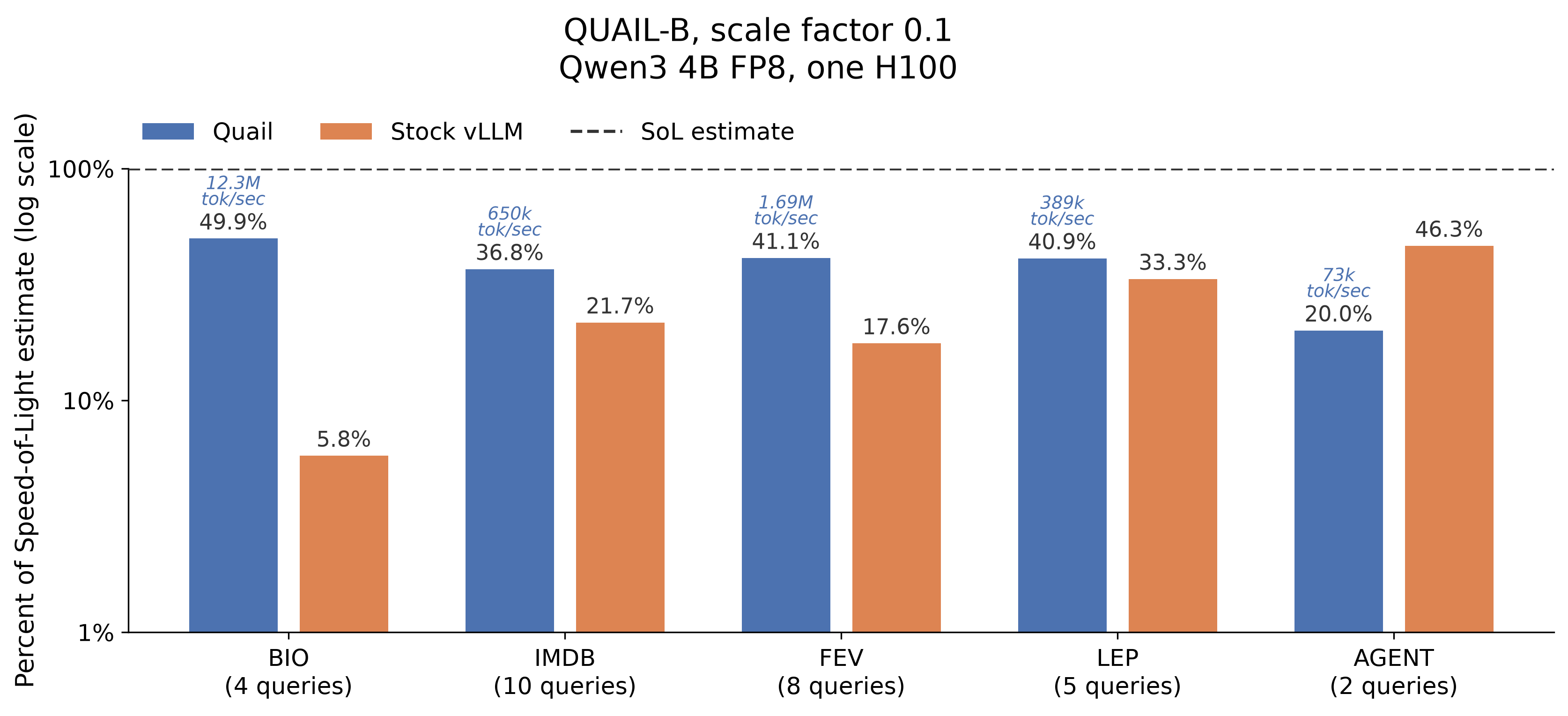
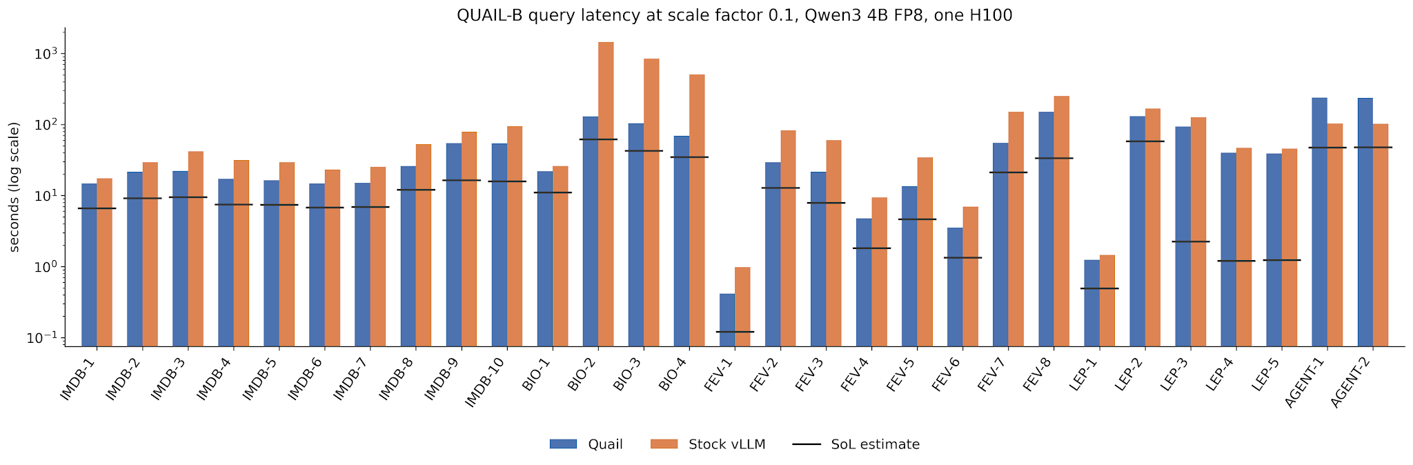
Figure 10 focuses on the eight queries where pipelining changes how vLLM submits requests. Pipelined vLLM is faster than stock vLLM on seven of them, by 1.12x on average and up to 1.27x on IMDB-6.
Stock vLLM is faster than Quail only on AGENT-1 and AGENT-2. Quail does not yet reuse matching prefixes across rows, so it recomputes far more KV tokens on each query. Section 4.4 examines AGENT-1.
4.3 Quail dominates vLLM on BIO-4: 14.04x faster!
BIO-4 contains the kind of reuse Quail currently handles well: long shared documents, two joins, and millions of related model calls whose order is known before execution. At scale factor 1.0, BIO-4 filters 5,000 medical reports and two uses of the same 4,144 reaction terms, then runs two joins over the surviving inputs.
Table 2 reports throughput, cost, and KV regret.
| Metric | Quail | Stock vLLM | SoL estimate |
|---|---|---|---|
| Requested input tokens/s | 19.03 million | 1.36 million | 37.37 million |
| GPU cost per query | $1.93 | $27.03 | $0.98 |
| KV regret | 18.0 million | 50.3 million | 0 (assumed) |
Table 2. BIO-4 results at scale factor 1.0. GPU cost excludes model startup. SoL values are estimates.
Quail takes 29.26 minutes, compared with 6.84 hours for stock vLLM. Quail is 14.04x faster. It is 1.96x the SoL estimate, while stock vLLM is 27.55x the estimate. Even with pipelining, vLLM still takes 4.00 hours.
Quail costs $1.93 per query, compared with $27.03 for stock vLLM. The SoL cost estimate is $0.98 per query. Quail processes 19.03 million requested input tokens per second, compared with 1.36 million for stock vLLM.
Quail also recomputes less KV. It recomputes 18.0 million tokens, compared with 50.3 million for stock vLLM.
4.4 But, vLLM dominates Quail on AGENT-1: Quail takes 2.32x as long.
AGENT-1 contains a different kind of reuse. It filters 1,772 cumulative snapshots from software agent runs. Separate rows contain overlapping prefixes from the same agent trace, and stock vLLM’s automatic prefix caching recognizes them. Quail does not yet recognize that relationship, so stock vLLM wins. Table 3 shows two example rows.
| id | trajectory_id | turn_index | trace |
|---|---|---|---|
| trace_42_turn_5 | trace_42 | 5 | [USER] Fix the failing parser. [ASSISTANT] Tries approach A. [TOOL] The test fails. |
| trace_42_turn_10 | trace_42 | 10 | <complete trace from turn 5> [ASSISTANT] Finds the mistake, and tries approach B. [TOOL] The tests pass. |
Table 3. Two cumulative snapshots from the same software agent trace.
Here is the AGENT-1 query, simplified for this post:
SELECT t.id
FROM agent_traces AS t
WHERE AI.IF(PROMPT(
    'Did the agent recover after trying an approach that did not work?\n\n{0}',
    t.trace
));
Table 4 reports throughput, cost, and KV regret.
| Metric | Quail | Stock vLLM | SoL estimate |
|---|---|---|---|
| Requested input tokens/s | 73,006 | 169,201 | 367,400 |
| GPU cost per query | $0.2623 | $0.1131 | $0.0521 |
| KV regret | 11,886,152 | 23,928 | 0 (assumed) |
Table 4. AGENT-1 results. GPU cost excludes model startup. SoL values are estimates.
Stock vLLM finishes AGENT-1 in 103.07 seconds, compared with Quail’s 239.12 seconds. Quail takes 2.32x as long. The SoL estimate is 47.47 seconds, so stock vLLM still takes 2.17x longer than the estimate.
Stock vLLM wins because its automatic prefix caching can reuse KV across rows with matching token prefixes. Quail currently reuses KV only when the same document appears again in the query, not across different documents. As a result, Quail incurs 11.89 million KV regret tokens, while stock vLLM incurs only 23,928.
We plan to add automatic prefix caching to Quail, but the lookup must remain cheap at the request volumes that AI-SQL queries can produce.
5. Put another way: Quail brings Jev-like speeds and intelligence to database-scale workloads.
Quail also supports DiffusionGemma 26B-A4B FP8, a larger mixture-of-experts model with 4B active parameters per token. This gives Quail a higher-intelligence option that is still extremely fast. On IMDB-2 at scale factor 0.1, DiffusionGemma matched 88.89% of Qwen3 32B’s answers, compared with 76.41% for Qwen3 4B. It ran the query in 32.41 seconds, or 1.53x as long as Qwen3 4B’s 21.20 seconds, on one H100.
This fits a broader class of workloads that need fast, bounded model decisions instead of long generated responses. Jev has highlighted the demand for this pattern in application backends. Quail targets its batch, online analytical processing (OLAP) version: one query creates thousands or millions of related decisions over a dataset, and Quail plans and runs them together. This makes Quail a good fit for LLM judge workflows, trace compaction, labeling, and other large-scale data transformations.
6. We are just getting started with Quail!
Some next steps are obvious. E.g., we want to support more AI-SQL operators, more models, and more hardware. We especially want to support tiny hybrid models, so you can run Quail on a MacBook.
We are also interested many research ideas fusing the database and inference worlds; here are just a few:
Use the full memory hierarchy for KV. Quail currently keeps reusable KV in GPU HBM or recomputes it. We want to move KV to host memory or local SSD when it does not fit on the GPU, then bring it back before reuse. We also want automatic prefix caching across rows. Perhaps we will also want to do KV compression (we know it is good to make indexes smaller).
Improve model FLOP/S utilization. Quail currently relies on DeepGEMM and FlashAttention for its main GPU kernels. We have not optimized the kernels themselves, and we are stoked to be working with Modal and Doubleword, inference experts, on kernel optimization.
Train models for execution and planning. Google’s work on lightweight proxy models for AI-SQL suggests small models can evaluate filters cheaply. The same models could predict selectivity and likely survivors for the query planner, helping Quail choose operator order and decide which KV to keep. The big systems question is how to run and train many specialized models alongside a larger model on the same GPU.
Can an AI join work like a hash join? Today, Quail reuses an anchor’s KV within one join loop, but it recomputes every partner for each new anchor. The same document is therefore encoded once per pair. Could we instead encode every document once and use its KV as a position-independent index entry? A document from the other relation could then search those entries for matches, like probing a hash table, without recomputing the indexed documents. This may require removing or separating the position information that RoPE adds to KV.
New methods for using AI agents to build systems. We used AI coding agents heavily to build the current version of Quail. We expect to keep using agents to build many of the features above. How do we do this correctly? We want better ways to specify what the system must do, and to check that every agent-written change keeps answers correct and runtime close to SoL. It feels inevitable that agents will do the bulk of the coding, and we are excited to build Quail in public and share the meta-learnings from building it with agents.
More blog posts, and eventually a technical report, are coming soon. For now, please try Quail! If these ideas sound interesting, reach out to get involved! And if you want to build an application on top of Quail, such as an LLM judge workflow in AI-SQL, Quail has an MIT license. It is now orders of magnitude cheaper to add intelligence to your data processing workflows, and we would love to see what you build :-)
Acknowledgements
We thank Modal for sponsoring the compute used in this research.
Notes
1. The query is based on the BioDEX
dataset. The SQL form
of BIO-4 is shown below. In each prompt, {0} and {1} refer to the first
and second arguments.
SELECT r.id,
    n.id AS neurological_reaction_id,
    c.id AS cardiovascular_reaction_id
FROM reports AS r
JOIN reaction_terms AS n
    ON AI.IF(PROMPT(
        'Does the medical report in {0} describe the reaction in {1} as '
        'something the patient experienced?',
        r.report,
        n.term
    ))
JOIN reaction_terms AS c
    ON AI.IF(PROMPT(
        'Does the medical report in {0} describe the reaction in {1} as '
        'something the patient experienced?',
        r.report,
        c.term
    ))
WHERE AI.IF(PROMPT(
    'Does {0} describe a serious or life-threatening adverse event?',
    r.report
))
AND AI.IF(PROMPT(
    'Is this reaction neurological, affecting the nervous system? {0}',
    n.term
))
AND AI.IF(PROMPT(
    'Is this reaction cardiovascular, affecting the heart or blood vessels? {0}',
    c.term
));
2. Prompts use numbered placeholders, such as {0} and {1}, to refer to
the arguments after the prompt string in the PROMPT call. The SQL call
and the model input it produces are shown below.
AI.IF(PROMPT(
    'Does {0} mention {1}?',
    r.report,
    n.term
))
The documents do not have to appear exactly where their placeholders occur in the question. Quail can place the report first so its KV can be reused when the same report is compared with another reaction term.
The model receives the following input:
DOCUMENT:
[contents of r.report]

(The document above is DOCUMENT {0}.)

Evaluate TRUE or FALSE for the following question:
Does {0} mention {1}?

DOCUMENT {1}:
[contents of n.term]
ANSWER:
Of course, whether other prompt layouts affect accuracy remains an open question, though we expect this to matter less as models improve.
3. The speed of light estimate assumes 100 percent model FLOP/s utilization (MFU), meaning every forward pass sustains the GPU’s peak arithmetic throughput. Real systems cannot reach that rate, so the estimate is an optimistic lower bound.
4. Modal provides useful background on GPU utilization and host overhead in inference engines.
5. The IMDB dataset was already on disk, so the measurement excludes the time and cost of downloading it.
6. We use OpenAI’s cached-token price in this estimate and assume an “infinite” cache, so every reusable document token receives that rate.
7. Marcel Rød built the fast Gigatoken tokenizer; thank you!
8. Kernel fusion can substantially improve prefill MFU. In “Chasing Speed of Light on TPU v6e,” Sail Research reports increasing Gemma 4 31B prefill MFU from about 32 percent to 63 percent through several optimizations, including folding activation, normalization, and RoPE work into surrounding kernels.
9. We follow a long line of “Tree”-based attention approaches, which evaluate several branches that share a prefix without allowing one branch to attend to another. E.g., SpecInfer uses a tree mask during speculative decoding to verify several possible continuations at once. Also, Hydragen uses shared-prefix attention during decoding to generate several outputs from one input. Quail applies the same structure, but during prefill.
10. One might expect two token IDs, one for each answer. For Qwen, Quail scores four spellings of each answer. The TRUE tokens are “TRUE” (20611), “␠TRUE” (8214), “True” (2514), and “␠True” (3007). The FALSE tokens are “FALSE” (30351), “␠FALSE” (7833), “False” (4049), and “␠False” (3557). Here, ␠ marks a leading space.
11. Both baselines use vLLM 0.26.0 with automatic prefix caching. We use the largest stable settings: 25,305 maximum batched tokens, 4,096 sequences, GPU memory utilization of 0.91, and one CUDA graph for 8,192 tokens. Larger settings ran out of GPU memory.
Cite this post
@misc{shankar2026quail,
  title = {Building an Ultra-High Throughput AI-SQL Engine},
  author = {Shankar, Shreya and Frye, Charles and Finn, Fergus and
            Dhariya, Arnav and Barrow, Joseph and Arik, Meryem},
  year = {2026},
  month = sep,
  url = {https://fsdatalab.github.io/blog/introducing-quail/}
}