Back to blog

How to Cost Your AI-Powered Filters

1. Introduction

We recently released Quail¹, an execution engine for AI-SQL, which extends SQL with functions that call LLMs. To choose between query plans, Quail needs to estimate how long each AI operation will take. But estimating AI operation latency is not straightforward! In this article, we discuss: How can we estimate the latency of an AI-SQL query on a given LLM and GPU?

One approach is to profile the system by running representative queries and fitting a model to the measurements. But such a profile would have to be redone for every new model, GPU, or workload, and might not even be accurate — which would be a massive headache. Instead, in Quail, we use the roofline model to estimate the latency of an AI operation.² That is, we compute the arithmetic and memory traffic needed for a query, then divide by the GPU’s peak compute throughput and memory bandwidth, to obtain a speed-of-light (SoL) estimate, or a lower bound on how quickly a query could run based on hardware limits.

In this article, we’ll walk through how to derive a SoL estimate for AI-SQL queries that only contain filter operators. Well go through:

• The GPU and transformer concepts behind our cost model (Section 2).
• How to estimate latency for one AI-powered filter (Section 3).
• How to cost a conjunction of filters and choose a filter order (Section 4).
• An example using Qwen3-4B-fp8 on an H100, with an interactive playground to explore different filter orders (Sections 5 and 6).

2. Background

Here, we first define AI-powered filters. We then describe the hardware and model choices used in our examples (H100 GPU and Qwen3-4B), giving an overview of the parts of a transformer forward pass that affect cost. Finally, we introduce the roofline model we use to estimate SoL latency.

2.1 AI-powered filters

We define AI-powered filters and introduce the single-filter query and the conjunction of filters used throughout the article.

AI-SQL filter. A regular SQL filter evaluates a condition such as price > 10. An AI-SQL filter instead asks an LLM to decide whether each row or document satisfies a condition written in natural language. To execute an AI-SQL filter, an LLM is invoked on each row or document and returns a single token, true or false.

Figure 1. An AI-SQL query applies three filters to four example IMDB reviews. The output shows the result of each filter. A dash in the expected output means that the filter was skipped because the review had already failed an earlier filter.

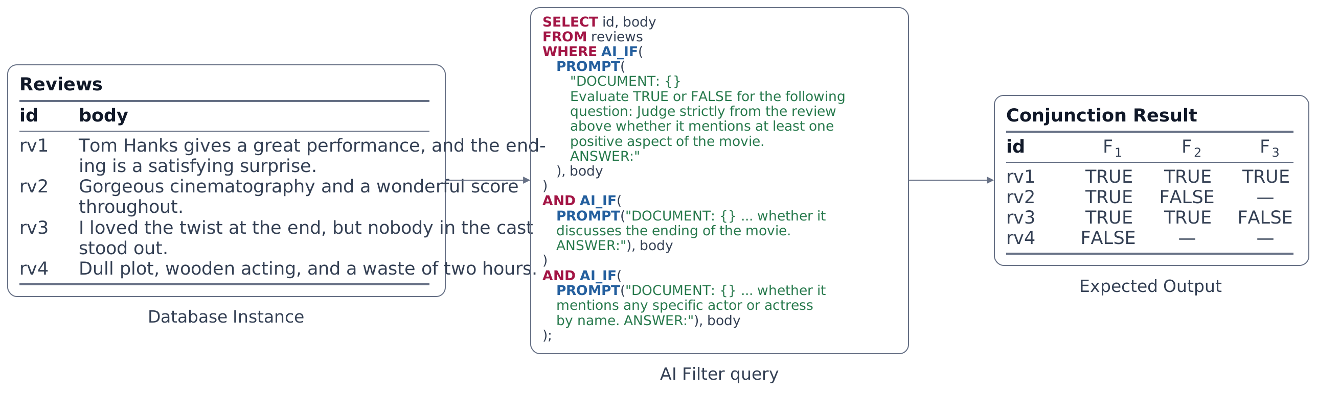
Figure 1 displays the general prompt structure for the AI-powered filter query; its structure is similar to that of a SQL query. Within each invocation of the operator there exists a preamble, “DOCUMENT:\n”, the actual document, and the filter instruction “Evaluate TRUE or FALSE for the following question: […]”. The output of each predicate is a single-token output of true or false. Only the surviving documents pass through to subsequent filters. Figure 1 shows a query with a conjunction of filters: \(F_1\) (mentions a positive aspect) → \(F_2\) (discusses the ending) → \(F_3\) (mentions a named actor), all three run over the reviews table. We use the first predicate as the single AI-powered filter example in Section 3.

The preamble and filter instruction add tokens to each request, so their lengths affect the cost.

2.2 GPU Execution

Our examples assume an NVIDIA H100 SXM GPU. Its Hopper architecture introduced FP8 Tensor Cores as part of a design aimed at accelerating transformer models.³ FP8 is an eight-bit floating-point number format.

Figure 2. H100 memory layout and forward-pass data movement.

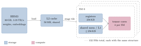
Figure 2 shows the parts of the H100 that affect our cost model. High-bandwidth memory (HBM) is the GPU’s main memory. It stores the model’s weight matrices, embedding table, and key-value (KV) cache, which holds attention vectors from previously processed tokens for reuse. We explain the vectors in Section 2.3. Data read from HBM passes through the shared L2 cache before being sent to one of the GPU’s 132 streaming multiprocessors (SMs). Within each SM, registers and the combined shared memory and L1 cache hold small tiles of data close to the Tensor Cores. Each SM has four Tensor Cores, which perform the matrix multiplications used by the model. The H100 has a 50 MB L2 cache shared by all of its SMs.

Our cost model tracks two hardware costs: arithmetic and HBM traffic. For arithmetic, it divides the number of floating-point operations (FLOPs) by the Tensor Core throughput. For HBM traffic, it divides the number of bytes read from or written to HBM by the HBM bandwidth. The model does not account for each intermediate cache level separately.

Table 1 maps the H100 specifications to the symbols used in our equations. Arithmetic throughput is the number of FLOPs that the GPU can perform per second, and memory bandwidth is the number of bytes that it can transfer from HBM per second. \(\Pi_{bf16}\) and \(\Pi_{fp8}\) are the peak arithmetic throughput rates for BF16 (a 16-bit floating-point number format) and FP8 operations, while \(\beta\) is the peak HBM bandwidth. We use the FP8 rate for the projection and MLP matrix multiplications, and the BF16 rate for attention in our FlashAttention⁴ setup.

Symbol	Value
\(\Pi_{bf16}\)	\(989.5\times10^{12}\) FLOP/s
\(\Pi_{fp8}\)	\(1.979\times10^{15}\) FLOP/s
\(\beta\)	\(3.35\times10^{12}\) bytes/s
Capacity	80 GB

Table 1. H100 SXM hardware constants.

2.3 Transformer Forward Pass

A forward pass processes input tokens through the model’s layers. Each filter processes its input and predicts one token, true or false. Within each layer, projections transform token vectors through matrix multiplication, attention combines information from the current and earlier tokens, and a multilayer perceptron (MLP) applies further transformations to each token independently. Our cost model counts the arithmetic and memory traffic of each component within every layer. We use Qwen3-4B FP8⁵ in our examples.⁶ The loaded model occupies about 4.5 GB in HBM.

Before the first layer, the model uses an embedding table to map each token ID to a hidden state, a vector of 2,560 values in Qwen3-4B. Each layer transforms the hidden state before passing it to the next layer.

Figure 3 shows the execution order within one Qwen3-4B layer. The model first computes query (Q), key (K), and value (V) projections, then performs attention and an output projection. The MLP follows.

Figure 3. A token passes through Q, K, and V projections, attention, an output projection, and the MLP. Attention also reads the K and V vectors of earlier tokens.

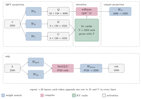
Projections. The model’s Q, K, and V projection matrices transform each token’s hidden state into Q, K, and V vectors used by attention. After attention, the output projection uses another matrix multiplication to produce a vector with the same width as the hidden state. Fortunately, projections can be highly parallelized: each projection applies the same matrix to every token independently, so the GPU can process many tokens at once. Processing more tokens together amortizes the cost of reading the weights from HBM, since the GPU can reuse the same weights across many tokens.

Attention. Attention combines the V vectors of the current token and earlier tokens. Comparing the current token’s Q vector with each token’s K vector determines how much each V vector contributes. Unfortunately, each token must be compared with itself and all previous tokens, so doubling the number of tokens roughly quadruples the attention arithmetic.

Models have multiple attention heads, and the attention calculation above runs separately for each head. Each head uses its own Q vector and computes its result independently, so the GPU can run the heads in parallel.

To reduce the memory needed for K and V, Qwen3-4B uses grouped query attention (GQA).⁷ Its 32 query heads are arranged in eight groups of four, and the heads in each group share the same K and V vectors. Sharing reduces the K and V projection matrices and KV cache to one quarter the size of full multi-head attention, where each of the 32 heads has its own K and V vectors.⁸

In Section 4, we will consider queries with multiple filters on the same document and explain how the filters can reuse the document’s cached K and V vectors (KV cache).

MLP. After attention and the output projection, the multilayer perceptron (MLP) further transforms each token’s hidden state. It first multiplies the hidden state by the gate and up matrices to produce two wider vectors. The SwiGLU activation first transforms the gate vector, then uses it to scale each element of the up vector.⁹ The down matrix then returns the result to the original hidden-state width. Like projections, the MLP operates on each token independently, so many tokens can run in parallel and share the weights read from HBM. Its arithmetic grows with the number of tokens, rather than the number of token pairs as in attention.

The resulting hidden states pass to the next transformer layer, which repeats the projections, attention, and MLP. Qwen3-4B has 36 layers. After the final layer, the model uses the same embedding table to convert the final hidden state into scores for output tokens. Table 2 lists the matrix dimensions and parameter counts we need to calculate the arithmetic and memory traffic across all layers.

Symbol	Meaning	Value
\(P\)	Non-embedding parameters	\(3.6\times10^{9}\)
layers	Transformer layers	36
\(d_{\text{model}}\)	Hidden-state width	2560
\(n_{\text{heads}}\)	Query heads	32
\(n_{\text{kv}}\)	Key-value heads	8
\(d_{\text{head}}\)	Width of each attention head	128
\(d_{\text{mlp}}\)	MLP intermediate width	9728
vocab	Vocabulary size	151936

Table 2. Qwen3-4B architecture constants.

The parameter count \(P\) includes only projection and MLP weights. The embedding table contains \(\text{vocab}\times d_{\text{model}}\) values, where \(\text{vocab}\) is the number of distinct tokens the model can read or output and \(d_{\text{model}}\) is the hidden-state width.

2.4 Roofline Model & Speed of Light

For each component of a forward pass, we need to estimate the time spent on arithmetic and memory transfers. The compute time is the number of FLOPs divided by the GPU’s arithmetic throughput. The memory transfer time is the number of bytes read from or written to HBM divided by the HBM bandwidth.

Sometimes arithmetic takes longer; other times, memory transfers take longer. We use the roofline model to estimate latency from both times. The model assumes that arithmetic and memory transfers overlap, so the component’s latency is the longer of the two:

\[T = \max\!\left(\frac{\text{FLOPs}}{\Pi},\; \frac{\text{Bytes Moved}}{\beta}\right).\]

Here, \(T\) is the estimated latency, \(\Pi\) is the arithmetic throughput in FLOP/s, and \(\beta\) is the HBM bandwidth in bytes/s. Using the GPU’s peak arithmetic throughput and memory bandwidth gives a speed-of-light (SoL) latency estimate for the operation. The estimate is a lower bound because an implementation may not sustain the peak rates or overlap arithmetic and memory transfers perfectly.

The roofline model predates modern LLMs. Williams et al. introduced it in 2009 to relate arithmetic and memory traffic to hardware performance. We learned a lot about applying it to transformer inference from blog posts by Kipply¹⁰, Fergus Finn¹¹, Ben Mayer¹², and Modal¹³, which we recommend reading.

If memory transfers take longer, the operation is memory-bound. If arithmetic takes longer, it is compute-bound. To determine which case applies, we compare the operation’s operational intensity, \(I\), with the GPU’s ridge point, \(I^*\):

\[I = \frac{\text{FLOPs}}{\text{Bytes Moved}}, \qquad I^* = \frac{\Pi}{\beta}.\]

Here, \(I\) is the arithmetic performed per byte transferred from HBM. \(I^*\) is the intensity at which compute time and memory transfer time are equal. Below the ridge point, the operation is memory-bound. Above it, the operation is compute-bound.

The H100 has different arithmetic throughput rates for FP8 and BF16, so each has a different ridge point. Our projections and MLP use FP8, while attention uses BF16. For the H100 rates in Table 1:

\[\begin{aligned} I^* &= \frac{\Pi_{fp8}}{\beta} = \frac{1.979\times10^{15}}{3.35\times10^{12}} \approx 590.75\ \text{FLOP/byte}, \\ I^*_{bf16} &= \frac{\Pi_{bf16}}{\beta} = \frac{989.5\times10^{12}}{3.35\times10^{12}} \approx 295.37\ \text{FLOP/byte}. \end{aligned}\]

Here, \(I^*\) is the FP8 ridge point used for projections and the MLP, and \(I^*_{bf16}\) is the BF16 ridge point used for attention.

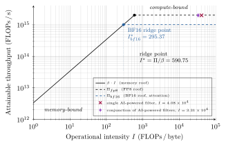
Figure 4 shows how operational intensity limits arithmetic throughput. In the sloped region, HBM bandwidth is the limit: performing more arithmetic for each byte transferred allows higher throughput. Once an operation reaches the ridge point, arithmetic throughput is the limit, so the plot becomes horizontal.

Figure 4. Roofline for an NVIDIA H100 SXM. The BF16 roof applies only to attention; × marks the single filter of Section 3, diamond marks the conjunction of Section 5.

In Section 3.5, we will calculate how many tokens we need to process before arithmetic, rather than memory transfers, determines each component’s latency.

3. Cost Model for One Filter

We estimate one filter’s latency by counting the arithmetic and memory traffic for projections, attention, and the MLP. We apply the roofline equation to each component and add the resulting latencies. Using one filter from our example query, we will calculate the cost of processing a batch of documents and predicting true or false for each document.

3.1 Workload and Notation

First, we will introduce notation for evaluating one filter on a batch of documents. A request is the input sent to the model for one document: the preamble, document, and filter instruction, in that order. We will describe the length of each request, the total number of tokens in the batch, and the number of forward passes needed to process them.

Let \(N\) be the number of documents in a batch and \(\ell_i\) the number of tokens in document \(i\). Let \(q_{\text{pre}}\) be the number of tokens in the preamble and \(q_{\text{tail}}\) the number of tokens in the filter instruction. We define the following quantities for the batch:

\[\begin{aligned} L_1 &= \sum_i \ell_i, \\ r_i &= q_{\text{pre}} + \ell_i + q_{\text{tail}}, \\ n_{\text{tok}} &= \sum_i r_i = L_1 + N(q_{\text{pre}} + q_{\text{tail}}), \\ L_2 &= \sum_i r_i^2. \end{aligned}\]

Here, \(L_1\) is the total number of document tokens in the batch. \(r_i\) is the full request length for document \(i\). \(n_{\text{tok}}\) is the total number of request tokens in the batch, including the preamble, document, and filter instruction in every request. \(L_2\) is the sum of the squared request lengths, which Section 3.3 uses to count attention comparisons.

Given that we estimate costs before executing the query, we can estimate the mean document length from a sample and use the mean in place of each \(\ell_i\). Using individual document lengths gives a tighter estimate, especially for attention, whose arithmetic depends on squared request lengths.

Then, let \(C\) be the token budget for one forward pass. We make \(C\) as large as possible so the GPU can reuse the weights across more tokens and read them from HBM fewer times. Quail sets \(C\) using the available HBM and the limits of its GPU programs, called kernels. For our Qwen3-4B example, the limiting constraint is the kernels’ 32-bit indexing. The token budget and the number of forward passes, \(K\), are

\[\begin{aligned} C &= \left\lfloor \frac{2^{31}-1}{2\,d_{\text{mlp}}} \right\rfloor, \\ K &= \left\lceil \frac{n_{\text{tok}}}{C} \right\rceil . \end{aligned}\]

Here, \(d_{\text{mlp}}\) is the MLP intermediate width from Table 2. Each token’s combined gate and up vectors occupy \(2d_{\text{mlp}}\) elements, so Quail’s 32-bit indexing limit of \(2^{31}-1\) elements determines \(C\). In Section 4.1, when we discuss multiple filters, the batch size will be further limited by the HBM available to retain documents’ KV caches.

3.2 Projection Cost

Here we derive the FLOPs for Q, K, V, and output projections, their HBM traffic across forward passes, and the projection roofline cost.

Q, K, V, and output projections are matrix multiplications over each token. Each matrix maps a vector of one width to another, so its parameter count is the product of its input and output widths. Per layer we have the following for each projection:

\[\begin{aligned} p_Q &= d_{\text{model}}\,n_{\text{heads}}\,d_{\text{head}}, \\ p_K &= d_{\text{model}}\,n_{kv}\,d_{\text{head}}, \\ p_V &= d_{\text{model}}\,n_{kv}\,d_{\text{head}}, \\ p_O &= n_{\text{heads}}\,d_{\text{head}}\,d_{\text{model}}. \end{aligned}\]

Here, \(p_Q\), \(p_K\), \(p_V\), and \(p_O\) are the parameter counts of the Q, K, V, and output projection matrices in one layer.

Thus, in every layer they hold \(2\,d_{\text{model}}\,d_{\text{head}}(n_{\text{heads}}+n_{kv})\) parameters. The totals for parameters, FLOPs, and memory transfer are given below along with the total projection cost.

\[\begin{aligned} P_{\text{proj}} &= \text{layers}\cdot 2\,d_{\text{model}}\,d_{\text{head}}(n_{\text{heads}}+n_{kv}), \\ F_{\text{proj}} &= 2\,P_{\text{proj}}\,n_{\text{tok}}, \\ B_{\text{proj}} &= b_w\,P_{\text{proj}}\,K, \\ T_{\text{proj}} &= \max\!\left(\frac{F_{\text{proj}}}{\Pi_{fp8}}, \frac{B_{\text{proj}}}{\beta}\right). \end{aligned}\]

Here, \(P_{\text{proj}}\) is the number of projection parameters across all layers. \(F_{\text{proj}}\) is the total number of projection FLOPs. For each token, we multiply each weight by an input value and add the product to the output sum, counting two FLOPs per weight. \(b_w\) is the number of bytes per weight, which is 1 for FP8. \(B_{\text{proj}}\) is the number of projection weight bytes read from HBM across all \(K\) forward passes. \(T_{\text{proj}}\) is the projection latency, which is the larger of compute time and memory transfer time.

3.3 Attention Cost

We now count attention’s arithmetic and memory traffic and use the roofline equation to estimate its latency.

Attention is different from the projections, as tokens here interact with each other. Each token attends to itself and to every earlier token in its own request. A request of \(r_i\) tokens makes \(1 + 2 + \dots + r_i - 1 + r_i\) comparisons, so across the batch

\[A = \sum_i \frac{r_i(r_i+1)}{2} = \frac{n_{\text{tok}} + L_2}{2},\]

Here, \(A\) is the total number of attention comparisons across the batch. \(n_{\text{tok}} = \sum_i r_i\) is the total number of request tokens, and \(L_2 = \sum_i r_i^2\) is the sum of the squared request lengths defined in Section 3.1.

One comparison, for one head in one layer, costs \(2\,d_{\text{head}}\) FLOPs for the dot product of Q and K vectors, because we do a multiply and addition per number, and another \(2\,d_{\text{head}}\) for the weighted sum over V vectors. Repeating across all \(n_{\text{heads}}\) and all layers gives,

\[F_{\text{attn}} = 4\,n_{\text{heads}}\,d_{\text{head}}\,\text{layers}\cdot A.\]

Here, \(F_{\text{attn}}\) is the total number of attention FLOPs across all heads and layers.

Unlike projections, attention has no weights of its own to read. Instead, attention uses the K and V vectors (KV) produced by the projections. For large batches, the KV vectors do not all fit in the GPU’s L2 cache, so they are stored in a temporary buffer in HBM.

Let \(B_{\text{kv}}\) be the bytes needed to store one token’s KV vectors across all layers, and \(b_{kv}\) the bytes per vector element (2 for BF16):

\[B_{\text{kv}} = 2\,b_{kv}\,\text{layers}\,n_{kv}\,d_{\text{head}},\]

The factor 2 accounts for one K vector and one V vector. Even though Qwen3-4B has 32 query heads, it stores only eight pairs of K and V vectors per token per layer, because every four query heads share a pair.

For a single filter, we write KV vectors for all \(n_{\text{tok}}\) input tokens. Our estimate of attention’s memory traffic, \(B_{\text{attn}}\), is therefore

\[B_{\text{attn}} = B_{\text{kv}}\,n_{\text{tok}}.\]

Let \(W\) count tokens whose new KV vectors we write and \(R\) count tokens whose saved KV vectors we read:

\[B_{\text{attn}} = B_{\text{kv}}\,(W + R).\]

For a single filter, \(W = n_{\text{tok}}\) and \(R = 0\) because no vectors have been saved by an earlier filter.¹⁴

Now, back to our roofline estimate. Our FlashAttention implementation uses BF16, so we use the H100’s BF16 arithmetic throughput:

\[T_{\text{attn}} = \max\!\left(\frac{F_{\text{attn}}}{\Pi_{bf16}}, \frac{B_{\text{attn}}}{\beta}\right).\]

Here, \(T_{\text{attn}}\) is the attention latency, which is the larger of compute time and memory transfer time.

3.4 MLP Cost

We still need to derive the FLOPs for the gate, up, and down MLP projections, their HBM traffic, and the MLP roofline cost.

The MLP acts on each token independently, so unlike attention its cost per token does not depend on the other tokens in the request. It has three matrices per layer, and the parameter count of each is the product of its input and output widths. \(W_{\text{gate}}\) and \(W_{\text{up}}\) map \(d_{\text{model}}\) to \(d_{\text{mlp}}\), while \(W_{\text{down}}\) maps \(d_{\text{mlp}}\) back to \(d_{\text{model}}\):

\[\begin{aligned} p_{\text{gate}} &= d_{\text{model}}\,d_{\text{mlp}}, \\ p_{\text{up}} &= d_{\text{model}}\,d_{\text{mlp}}, \\ p_{\text{down}} &= d_{\text{mlp}}\,d_{\text{model}}. \end{aligned}\]

Here, \(p_{\text{gate}}\), \(p_{\text{up}}\), and \(p_{\text{down}}\) are the parameter counts of the gate, up, and down matrices in one layer.

Gate and up read the same input; their outputs are combined by SwiGLU (Swish Gated Linear Unit) activation and projected back down. The total parameters in the MLP are,

\[P_{\text{mlp}} = \text{layers}\cdot(p_{\text{gate}} + p_{\text{up}} + p_{\text{down}}) = 3\,\text{layers}\,d_{\text{model}}\,d_{\text{mlp}}.\]

Here, \(P_{\text{mlp}}\) is the number of MLP parameters across all layers.

The reasoning for the MLP is the same as it is for the projections: every token is multiplied by every weight once, and the weights are streamed from HBM once per forward pass.

\[\begin{aligned} F_{\text{mlp}} &= 2\,P_{\text{mlp}}\,n_{\text{tok}}, \\ B_{\text{mlp}} &= b_w\,P_{\text{mlp}}\,K. \end{aligned}\]

Here, \(F_{\text{mlp}}\) is the total number of MLP FLOPs. \(B_{\text{mlp}}\) is the number of MLP weight bytes read from HBM across all \(K\) forward passes.

The MLP matrix multiplications use FP8, so the roofline estimate uses the H100’s FP8 arithmetic throughput:

\[T_{\text{mlp}} = \max\!\left(\frac{F_{\text{mlp}}}{\Pi_{fp8}}, \frac{B_{\text{mlp}}}{\beta}\right).\]

Here, \(T_{\text{mlp}}\) is the MLP latency, which is the larger of compute time and memory transfer time.

3.5 Total Cost

A forward pass runs the projections, attention, and the MLP in sequence, so the three component times add:

\[T_{\text{filter}} = T_{\text{proj}} + T_{\text{attn}} + T_{\text{mlp}}.\]

Here, \(T_{\text{filter}}\) is the total latency of one filter.

We will go through the following questions to give you some intuition for how batch size and request length affect latency.

When do projections and the MLP become compute-bound?

For either projections or the MLP, let \(P\) be the component’s weight count. Section 3.2 and Section 3.4 give \(2P n_{\text{tok}}\) FLOPs and \(b_w P K\) bytes of weight reads. With FP8 weights, \(b_w = 1\), so the operational intensity, \(I\), is

\[I = \frac{2P n_{\text{tok}}}{b_w P K} = 2\,\frac{n_{\text{tok}}}{K}.\]

The weight count cancels, leaving twice the average number of tokens per forward pass. The factor 2 counts the multiplication and addition performed for each weight and token.¹⁵ To exceed the H100’s FP8 ridge point of about 591 FLOPs per byte, we need only about 296 tokens per forward pass. Batch-processing workloads typically exceed that threshold, so projections and the MLP are compute-bound.

When does attention dominate latency?

Once the components are compute-bound, we can compare their arithmetic times directly. From the earlier roofline formulas,

\[\begin{aligned} T_{\text{proj}} + T_{\text{mlp}} &\approx \frac{2(P_{\text{proj}}+P_{\text{mlp}})\,n_{\text{tok}}}{\Pi_{fp8}}, \\ T_{\text{attn}} &\approx \frac{4\,n_{\text{heads}}\,d_{\text{head}}\,\text{layers}\,A}{\Pi_{bf16}}. \end{aligned}\]

Projection and MLP arithmetic grows with the number of tokens; attention arithmetic grows with the number of token pairs. If every request contains \(r\) tokens, then \(n_{\text{tok}} = Nr\) and \(A = Nr(r+1)/2\). Dividing the attention time by the combined projection and MLP time gives

\[\begin{aligned} \frac{T_{\text{attn}}}{T_{\text{proj}}+T_{\text{mlp}}} &\approx \frac{n_{\text{heads}}\,d_{\text{head}}\,\text{layers}\,(r+1)} {P_{\text{proj}}+P_{\text{mlp}}} \cdot \frac{\Pi_{fp8}}{\Pi_{bf16}} \\ &= \frac{r+1}{12{,}320}. \end{aligned}\]

With our model and hardware specs, projections and MLPs dominate the estimated latency for requests shorter than about 12,300 tokens. Above that length, attention dominates.

3.6 Cost of One IMDB Filter

We can finally estimate the SoL latency of applying \(F_1\), the filter that asks whether a review mentions a positive aspect of the movie, to 5,000 IMDB reviews! This is the first filter in Figure 1. We use the H100 specs, along with the following batch and prompt values:

\[N = 5{,}000, \qquad \bar{\ell} = 298.8466 \ \text{tokens}, \qquad q_{\text{pre}} = 2 \ \text{tokens}, \qquad q_{\text{tail}} = 51 \ \text{tokens}.\]

Here, \(N\) is the number of reviews, \(\bar{\ell}\) is the mean review length, \(q_{\text{pre}}\) is the preamble length, and \(q_{\text{tail}}\) is the length of \(F_1\)’s instruction.

We approximate every document by the mean length, which gives

\[L_1 = N\bar{\ell} = 1{,}494{,}233 \ \text{tokens}.\]

Request and batch sizes. Each request contains the preamble, one document, and the filter instruction:

\[\begin{aligned} r &= q_{\text{pre}} + \bar{\ell} + q_{\text{tail}} = 2 + 298.8466 + 51 = 351.8466 \ \text{tokens}, \\ n_{\text{tok}} &= N r = 5{,}000 \times 351.8466 = 1{,}759{,}233. \end{aligned}\]

Here, \(r\) is the common request length under the mean-length approximation. \(n_{\text{tok}}\) is the total number of request tokens across all 5,000 reviews.

Attention comparisons. The attention calculation also needs the sum of squared request lengths:

\[\begin{aligned} L_2 &= N r^2 = 5{,}000 \times 351.8466^2 = 618{,}980{,}149.66, \\ A &= \frac{n_{\text{tok}} + L_2}{2} = 310{,}369{,}691.33 . \end{aligned}\]

Here, \(L_2\) is the sum of the squared request lengths, and \(A\) is the total number of attention comparisons. Using the mean length for every request underestimates attention arithmetic when review lengths vary, because the mean of squared lengths is larger than the square of the mean length.

Forward passes. Using the token budget from Section 3.1, \(C = 110{,}376\), processing all 5,000 reviews requires

\[K = \left\lceil \frac{1{,}759{,}233}{110{,}376} \right\rceil = 16 \text{ forward passes}.\]

Model parameters. We substitute the Qwen3-4B dimensions from Table 2:

\[\begin{aligned} d_{\text{model}} &= 2560, & d_{\text{mlp}} &= 9728, & d_{\text{head}} &= 128, \\ n_{\text{heads}} &= 32, & n_{kv} &= 8, & \text{layers} &= 36. \end{aligned}\] \[\begin{aligned} P_{\text{proj}} &= 36 \cdot 2 \cdot 2560 \cdot 128 \cdot (32+8) = 943{,}718{,}400, \\ P_{\text{mlp}} &= 3 \cdot 36 \cdot 2560 \cdot 9728 = 2{,}689{,}597{,}440 . \end{aligned}\]

Projections.

\[\begin{aligned} F_{\text{proj}} &= 2 \times 943{,}718{,}400 \times 1{,}759{,}233 \\ &\approx 3.3204\times10^{15}\ \text{FLOPs},\\[0.4em] B_{\text{proj}} &= 1 \times 943{,}718{,}400 \times 16 \\ &\approx 1.5099\times10^{10}\ \text{bytes},\\[0.4em] T_{\text{proj}} &= \max\!\left( \frac{3.3204\times10^{15}}{1.979\times10^{15}}, \frac{1.5099\times10^{10}}{3.35\times10^{12}} \right)\\[0.3em] &= \max(1.6778,\ 0.0045) = 1.6778\ \text{s}. \end{aligned}\]

Attention.

\[\begin{aligned} F_{\text{attn}} &= 4 \times 32 \times 128 \times 36 \times A \\ &= 589{,}824 \times 310{,}369{,}691.33 \\ &\approx 1.8306\times10^{14}\ \text{FLOPs},\\[0.4em] B_{\text{kv}} &= 2 \times 2 \times 36 \times 8 \times 128 \\ &= 147{,}456\ \text{bytes/token},\\[0.4em] B_{\text{attn}} &= 147{,}456 \times (1{,}759{,}233 + 0) \\ &\approx 2.5941\times10^{11}\ \text{bytes},\\[0.4em] T_{\text{attn}} &= \max\!\left( \frac{1.8306\times10^{14}}{989.5\times10^{12}}, \frac{2.5941\times10^{11}}{3.35\times10^{12}} \right)\\[0.3em] &= \max(0.1850,\ 0.0774) = 0.1850\ \text{s}. \end{aligned}\]

MLP.

\[\begin{aligned} F_{\text{mlp}} &= 2 \times 2{,}689{,}597{,}440 \times 1{,}759{,}233 \\ &\approx 9.4633\times10^{15}\ \text{FLOPs},\\[0.4em] B_{\text{mlp}} &= 1 \times 2{,}689{,}597{,}440 \times 16 \\ &\approx 4.3034\times10^{10}\ \text{bytes},\\[0.4em] T_{\text{mlp}} &= \max\!\left( \frac{9.4633\times10^{15}}{1.979\times10^{15}}, \frac{4.3034\times10^{10}}{3.35\times10^{12}} \right)\\[0.3em] &= \max(4.7818,\ 0.0128) = 4.7818\ \text{s}. \end{aligned}\]

Total.

\[\begin{aligned} T_{\text{filter}} &= T_{\text{proj}} + T_{\text{attn}} + T_{\text{mlp}} \\ &= 1.6778 + 0.1850 + 4.7818 \\ &= \boxed{6.64\ \text{seconds}}. \end{aligned}\]

Component	FLOPs	Bytes	\(T_{\text{compute}}\)	\(T_{\text{memory}}\)
Projections	\(3.32\times10^{15}\)	\(1.51\times10^{10}\)	1.6778 s	0.0045 s
Attention	\(1.83\times10^{14}\)	\(2.59\times10^{11}\)	0.1850 s	0.0774 s
MLP	\(9.46\times10^{15}\)	\(4.30\times10^{10}\)	4.7818 s	0.0128 s
Total	\(1.30\times10^{16}\)	\(3.17\times10^{11}\)	6.64 s	0.09 s

Table 3. Estimated cost of applying F₁ (mentions a positive aspect) to all 5,000 IMDB reviews on Qwen3-4B and an H100. Every component is compute-bound.

The estimated SoL latency is 6.64 seconds for all 5,000 reviews, not for one review! So fast!

4. Cost Model for a Conjunction of Filters

Now let’s estimate the cost of applying several filters to the same documents. We can skip later filters for a document that fails, and reuse the document’s KV vectors if it passes. First, we will find a batch size that lets us keep the KV vectors in HBM. Then we will compare filter orders using their per-document costs. Finally, we will derive the SoL estimate for the selected order.

4.1 KV Reuse and HBM Capacity

Taking a closer look at Figure 1, every filter prompt for a given document contains the same preamble and document. Only the filter instruction changes. We call the shared preamble and document the prefix. Its average length, \(p\), is

\[p = q_{\text{pre}} + \bar{\ell}.\]

The first filter computes the prefix’s KV vectors. Later filters reuse them and process only their own instruction tokens. Our cost model assumes the saved vectors remain in HBM until the document fails a filter or passes the final filter. We therefore choose a batch whose prefix KV vectors fit in HBM.

HBM available for KV. The GPU needs space for model weights, temporary intermediate vectors called activations, and saved KV vectors. We use a rough estimate of peak activation memory.¹⁶ Inference engines such as vLLM instead run a forward pass with dummy inputs to profile peak activation memory before determining how much space remains for KV.

Quail makes 95% of the H100’s 80 GB available to its memory pool. Let \(M_{\text{KV}}\) be the space left for saved KV vectors after accounting for resident weights, including the embedding table and any extra storage required by FP8 weights, and temporary buffers:

\[M_{\text{KV}} = \text{usable HBM} - \text{resident weights} - \text{temporary buffers}.\]

Table 4 gives the resulting budget for our example.

Item	Size (GB)
Usable HBM (95% of 80 GB)	76.00
− Resident weights	4.50
− Estimated temporary buffers	18.08
Left for KV cache	53.42

Table 4. Estimated HBM budget for Qwen3-4B on an H100 SXM.

Batch size in documents. Section 3.3 gives \(B_{\text{kv}} = 147{,}456\) bytes per token. With an average prefix length of \(p = 300.8466\) tokens, one document’s prefix KV takes about 44.4 MB. Let \(N_b\) be the maximum number of documents in a batch whose KV vectors fit in HBM. Unlike \(C\), which counts tokens per forward pass, \(N_b\) counts documents. We divide the available KV memory by the bytes needed for one document’s prefix:

\[N_b = \left\lfloor \frac{M_{\text{KV}}}{B_{\text{kv}}\,p} \right\rfloor \approx 1{,}200\ \text{documents}.\]

We therefore split the 5,000 reviews into five batches. Because the bound uses the mean document length, it is an estimate rather than a guarantee for every batch.

4.2 Cost of a Fixed Filter Order

Suppose a query applies \(m\) filters to \(N\) documents. We write the filter order as \(\pi\), a list of filters. For example, \(\pi=(F_2,F_1,F_3)\) means we evaluate \(F_2\) first, then \(F_1\), then \(F_3\). The symbol \(\pi_j\) denotes the filter in position \(j\), so in this example \(\pi_1=F_2\), \(\pi_2=F_1\), and \(\pi_3=F_3\).

Selectivity, \(s_i\), is the fraction of documents that pass filter \(F_i\). Let \(N_j\) be the expected number of documents evaluated by the filter in position \(j\). We evaluate that filter only on documents that pass every preceding filter:¹⁷

\[N_j = N \prod_{k<j} s_{\pi_k}.\]

As in Section 3, we count the tokens processed \(n\), attention comparisons \(A\), tokens whose KV vectors are written \(W\), and tokens whose saved KV vectors are read \(R\). We shorten \(n_{\text{tok}}\) to \(n\) here and use \(n_j\) for the tokens processed by the filter in position \(j\).

First filter. Let \(q_i\) be filter \(F_i\)’s instruction length, corresponding to \(q_{\text{tail}}\) in the single-filter model. We write \(q_{\pi_j}\) for the instruction length of the filter in position \(j\). Using document lengths \(\ell_i\) from Section 3.1, the first request for document \(i\) has length \(r_i = q_{\text{pre}} + \ell_i + q_{\pi_1}\). The first filter processes all \(N\) documents:

\[\begin{aligned} n_1 &= \sum_{i=1}^{N} r_i, \\ A_1 &= \sum_{i=1}^{N}\frac{r_i(r_i+1)}{2}, \\ W_1 &= n_1, \\ R_1 &= 0. \end{aligned}\]

Here, \(n_1\) is the number of tokens processed, \(A_1\) is the number of attention comparisons, and \(W_1\) is the number of tokens whose new KV vectors are written. No saved KV vectors are available to read, so \(R_1 = 0\).

Later filters. At position \(j>1\), we process only the instruction tokens for the \(N_j\) surviving documents.¹⁸ Each instruction token attends to the cached prefix of average length \(p\) and to itself and earlier instruction tokens:

\[\begin{aligned} n_j &= N_j\,q_{\pi_j}, \\ A_j &= N_j\left[q_{\pi_j}\,p + \frac{q_{\pi_j}(q_{\pi_j}+1)}{2}\right], \\ W_j &= n_j, \\ R_j &= N_j\,p. \end{aligned}\]

Here, \(n_j\) is the number of instruction tokens processed, \(A_j\) is the number of attention comparisons, \(W_j\) counts tokens whose new KV vectors are written, and \(R_j\) counts tokens whose saved KV vectors are read. In \(A_j\), the first term counts comparisons with the prefix and the second counts comparisons within the instruction.

From work to cost. Write \(T_{\text{filter}}(n,A,W,R)\) for the latency obtained by substituting the workload counts into the equations from Section 3. For comparing orders, we assume full forward passes and use \(K=n/C\).

The scan cost is the first filter’s latency per document. The ask cost is a later filter’s latency per surviving document. Using the counts above,

\[\begin{aligned} \text{scan}_{\pi_1} &= \frac{T_{\text{filter}}(n_1,A_1,W_1,R_1)}{N}, \\[0.8em] \text{ask}_{\pi_j} &= \frac{T_{\text{filter}}(n_j,A_j,W_j,R_j)}{N_j}, \qquad j>1,\ N_j>0. \end{aligned}\]

If no documents reach a filter, it adds no cost.

The first filter incurs its scan cost for all \(N\) documents. Each later filter incurs its ask cost for the \(N_j\) documents that reach it. We add these costs to obtain an ordering score, \(S(\pi)\):

\[S(\pi) = N\,\text{scan}_{\pi_1} + \sum_{j=2}^{m} N_j\,\text{ask}_{\pi_j}.\]

4.3 Choosing the Filter Order

We now choose the order with the lowest ordering score. Our ordering rule follows Joseph Hellerstein and Michael Stonebraker’s work on ordering expensive predicates.¹⁹ For filters after the first position, we rank each filter by its ask cost per document rejected:

\[\text{rank}_i = \frac{\text{ask}_i}{1-s_i}.\]

Here, \(\text{rank}_i\) divides the filter’s ask cost by the fraction of documents it rejects. Lower ranks favor filters that reject more documents for less cost. If a filter passes every document (\(s_i=1\)), we set \(\text{rank}_i=\infty\).

Algorithm 1. Filter ordering (pseudocode).

\(\sigma \leftarrow\) filters sorted by ascending rank

for each filter \(F_i\):

\(\pi^{(i)} \leftarrow\) \(F_i\), followed by the filters in \(\sigma\) except \(F_i\)

evaluate \(S(\pi^{(i)})\) using the equation in Section 4.2

return the candidate \(\pi^{(i)}\) with the lowest \(S(\pi^{(i)})\)

Here, \(\sigma\) is the rank-sorted order, and \(\pi^{(i)}\) is the candidate order with filter \(F_i\) first. The superscript is the first filter’s number, while \(\pi_j\) denotes the filter in position \(j\). Algorithm 1 sorts only once and preserves the rank order of the remaining filters in each candidate.

For example, if sorting by rank gives \(\sigma=(F_2,F_1,F_3)\), the candidates are

\[\begin{aligned} \pi^{(2)}&=(F_2,F_1,F_3),\\ \pi^{(1)}&=(F_1,F_2,F_3),\\ \pi^{(3)}&=(F_3,F_2,F_1). \end{aligned}\]

The selected order, \(\pi_{\text{opt}}\), is

\[\pi_{\text{opt}} = \underset{\pi\,\in\,\{\pi^{(1)},\ldots,\pi^{(m)}\}}{\arg\min}\ S(\pi).\]

We sort the filters once in \(O(m\log m)\) time. After sorting, Quail computes each candidate’s score in constant time, so choosing among all \(m\) candidates takes \(O(m\log m)\) overall.

Proof sketch: why Algorithm 1 minimizes \(S(\pi)\)

Assume fixed, nonnegative scan and ask costs per document, and selectivities that do not change with filter order.

Fix the first filter. Let \(i\) and \(j\) be adjacent filters after the first, and let \(D\) be the expected number of documents evaluated by the earlier of the two. Their contribution to \(S(\pi)\) is \(D(\text{ask}_i+s_i\text{ask}_j)\) if \(i\) runs first, or \(D(\text{ask}_j+s_j\text{ask}_i)\) if \(j\) runs first. Either order leaves \(Ds_i s_j\) documents on average, so swapping the pair changes no other filter’s cost.

Swapping \(j,i\) to \(i,j\) changes \(S(\pi)\) by

\[D\left[\text{ask}_i(1-s_j)-\text{ask}_j(1-s_i)\right].\]

For \(s_i,s_j<1\), the change is nonpositive whenever

\[\text{rank}_i =\frac{\text{ask}_i}{1-s_i} \le \frac{\text{ask}_j}{1-s_j} =\text{rank}_j.\]

If \(s_j=1\), the change is \(-D\,\text{ask}_j(1-s_i)\le 0\), so placing \(j\) after \(i\) cannot increase the score. If both selectivities are 1, either order has the same cost. Filters with selectivity 1 can therefore go last, as prescribed by their infinite ranks.

Sorting the remaining filters by adjacent swaps cannot increase \(S(\pi)\), so rank order is optimal for any fixed first filter. Algorithm 1 tries every first filter and selects the lowest-scoring candidate, hence minimizes \(S(\pi)\) over all orders.

SoL latency of the selected order. The cost model we use for query planning, which we have described so far, is pretty simple. However, an astute reader will notice that the ordering score \(S(\pi)\) charges each filter separately. It does not allow arithmetic for one filter to overlap with memory transfers for another filter.

To see why, suppose attention for the first filter requires 10 ms of arithmetic and 1 ms of memory transfers, while attention for a later filter requires 1 ms of arithmetic and 5 ms of memory transfers. Applying our cost model gives

\[\max(10,1) + \max(1,5) = 15~\text{ms}.\]

But across both filters, attention requires 11 ms of arithmetic and 6 ms of memory transfers. Applying the roofline equation to the combined attention gives a lower estimate:

\[\max(10+1,\;1+5) = 11~\text{ms}.\]

Achieving 11 ms would require overlapping arithmetic and memory transfers across filters, for example by pipelining documents within each batch across filters. Nevertheless, to calculate this lower bound, we first count the tokens and attention comparisons across all filters in the selected order.²⁰

Let \(n\) be the total number of tokens processed and \(A\) the total number of attention comparisons. We also total the KV traffic, with \(W\) counting tokens whose new KV vectors are written and \(R\) counting tokens whose saved KV vectors are read:

\[\begin{aligned} n &= \sum_{j=1}^{m} n_j, & A &= \sum_{j=1}^{m} A_j, \\ W &= \sum_{j=1}^{m} W_j, & R &= \sum_{j=1}^{m} R_j. \end{aligned}\]

For the query’s SoL latency estimate, we round up the forward-pass count, \(K=\lceil n/C\rceil\). Substituting the totals into the projection, attention, and MLP formulas from Section 3 gives the query’s estimated SoL latency, \(T_{\text{query}}\):

\[\begin{aligned} T_{\text{query}} &= \max\!\left( \frac{2P_{\text{proj}}n}{\Pi_{fp8}},\; \frac{b_w P_{\text{proj}}K}{\beta} \right) \\ &\quad + \max\!\left( \frac{4n_{\text{heads}}d_{\text{head}}\,\text{layers}\,A}{\Pi_{bf16}},\; \frac{B_{\text{kv}}(W+R)}{\beta} \right) \\ &\quad + \max\!\left( \frac{2P_{\text{mlp}}n}{\Pi_{fp8}},\; \frac{b_w P_{\text{mlp}}K}{\beta} \right). \end{aligned}\]

5. Example: IMDB Query

Here we walk through our cost model for the example query over \(N=5{,}000\) IMDB reviews²¹ using Qwen3-4B on an H100. We first calculate the ordering score \(S(\pi)\) for each candidate from Algorithm 1. We then calculate the SoL latency \(T_{\text{query}}\) for the selected order, \(F_2 \to F_1 \to F_3\).

The weights use FP8, while attention and KV use BF16. The cached prefix contains \(p = 2 + 298.8466 = 300.8466\) tokens per review.

5.1 Filter Ordering

Table 5 lists the three filters. We assume we know each filter’s selectivity, the fraction of reviews that pass it.

We calculate scan and ask costs per document using the equations from Section 4.2, the H100 specs in Table 1, and the Qwen3-4B constants in Table 2. As in the planning model, we assume tokens are packed into full forward passes. Projections and the MLP are compute-bound at our token budget, so their latency estimates use the arithmetic times.

We will calculate both costs for \(F_1\), which asks whether a review mentions a positive aspect. Its ask cost applies when it runs after another filter, and its scan cost applies when it runs first.

Ask cost. When \(F_1\) runs after another filter, it processes only its instruction. Let \(q=q_1=51\) be the instruction’s token count. The projection arithmetic per document takes

\[T_{\text{proj}} = \frac{2 \times 943{,}718{,}400 \times 51}{1.979\times10^{15}} = 0.0486~\text{ms},\]

The MLP arithmetic takes

\[T_{\text{mlp}} = \frac{2 \times 2{,}689{,}597{,}440 \times 51}{1.979\times10^{15}} = 0.1386~\text{ms},\]

For attention, each of the 51 new tokens attends to the \(p\) cached tokens, itself, and earlier instruction tokens. The number of attention comparisons per document is

\[A = q\,p + \frac{q(q+1)}{2} = 51 \times 300.8466 + \frac{51 \times 52}{2} = 16{,}669.18.\]

Attention reads the saved KV vectors for \(p\) tokens and writes new KV vectors for \(q\) tokens. With \(W+R=p+q=351.8466\), its latency estimate is

\[\begin{aligned} T_{\text{attn}} &= \max\!\left( \frac{589{,}824 \times 16{,}669.18}{989.5\times10^{12}},\; \frac{147{,}456 \times 351.8466}{3.35\times10^{12}}\right) \\ &= \max(0.0099,\ 0.0155)~\text{ms} = 0.0155~\text{ms}, \end{aligned}\]

Memory transfers take longer than arithmetic for attention. Adding the three component latencies gives the ask cost per document:

\[\text{ask}_1 = T_{\text{proj}} + T_{\text{mlp}} + T_{\text{attn}} = 0.0486 + 0.1386 + 0.0155 = 0.203~\text{ms}.\]

Scan cost. When \(F_1\) runs first, it processes the preamble, review, and instruction. The full request contains \(r=p+q=351.8466\) tokens. The projection arithmetic per document takes

\[T_{\text{proj}} = \frac{2 \times 943{,}718{,}400 \times 351.8466}{1.979\times10^{15}} = 0.336~\text{ms},\]

The MLP arithmetic takes

\[T_{\text{mlp}} = \frac{2 \times 2{,}689{,}597{,}440 \times 351.8466}{1.979\times10^{15}} = 0.956~\text{ms},\]

The number of attention comparisons per document is

\[A = \frac{r(r+1)}{2} = \frac{351.8466 \times 352.8466}{2} = 62{,}073.94\]

The attention arithmetic therefore takes

\[T_{\text{attn}} = \frac{589{,}824 \times 62{,}073.94}{989.5\times10^{12}} = 0.0370~\text{ms},\]

We write new KV vectors for all \(r\) tokens and read no vectors saved by an earlier filter, so \(W=r\) and \(R=0\). The memory transfer time is

\[\frac{147{,}456 \times 351.8466}{3.35\times10^{12}} = 0.0155~\text{ms},\]

Arithmetic takes longer than memory transfers for attention, so the scan cost per document is

\[\text{scan}_1 = 0.336 + 0.956 + 0.037 = 1.329~\text{ms}.\]

We calculate the other filters’ costs the same way, using 45 instruction tokens for \(F_2\) and 49 for \(F_3\).

Filter	Predicate	\(q_i\)	\(s_i\)	\(\text{ask}_i\) (ms)	\(\text{scan}_i\) (ms)	\(1-s_i\)	rank (ms)
\(F_2\)	discusses the ending	45	0.2273	0.180	1.306	0.7727	0.234
\(F_1\)	mentions a positive aspect	51	0.4856	0.203	1.329	0.5144	0.394
\(F_3\)	mentions a named actor	49	0.6123	0.195	1.321	0.3877	0.504

Table 5. Filters sorted by ascending rank ask_i/(1−s_i). Each s_i is the assumed fraction of reviews that pass the filter.

Sorting by rank gives \(F_2 \to F_1 \to F_3\), rather than the written order \(F_1 \to F_2 \to F_3\). The ask costs differ by only about 13% because the instructions have similar lengths. \(F_2\) rejects the most documents per unit of estimated latency, while \(F_3\) rejects the fewest, so \(F_3\) goes last. To compare orders, we assume each filter keeps the same fraction of documents regardless of which filters ran before it.

We still need to compare each possible first filter, as described in Section 4.3. Table 6 shows that starting with \(F_2\) gives the lowest ordering score. Starting with \(F_1\) costs \(0.324\) s, or about 4.7%, more. Its scan is more expensive, and it passes about 2,428 documents to \(F_2\). Starting with \(F_2\) passes only about 1,137 documents to \(F_1\).

For the candidate \(\pi=(F_2,F_1,F_3)\), the expected numbers of reviews evaluated by each filter are

\[\begin{aligned} N_1&=5{,}000,\\ N_2&=5{,}000\times s_2=1{,}136.5,\\ N_3&=5{,}000\times s_2\times s_1=551.8844. \end{aligned}\]

Substituting the counts and the scan and ask costs into \(S(\pi)\) from Section 4.2 gives

\[\begin{aligned} S((F_2,F_1,F_3)) &=5{,}000\,\text{scan}_2 +1{,}136.5\,\text{ask}_1 +551.8844\,\text{ask}_3\\ &\approx 6.8665~\text{s}. \end{aligned}\]

We use unrounded scan and ask costs when calculating the scores. Table 6 compares the candidates from Algorithm 1.

First	Ordering \(\pi\)	\(S(\pi)\) (s)
\(F_2\)	\(F_2 \to F_1 \to F_3\)	6.8665
\(F_1\)	\(F_1 \to F_2 \to F_3\)	7.1906
\(F_3\)	\(F_3 \to F_2 \to F_1\)	7.2994

Table 6. Ordering score for each candidate ordering.

We select \(F_2 \to F_1 \to F_3\), which has the lowest ordering score, \(S(\pi)=6.8665\) s.

5.2 SoL Estimate for the Ordered Conjunction

We now calculate \(T_{\text{query}}\) for the same order, \(\pi=(F_2,F_1,F_3)\), using the query-wide roofline equation from Section 4.3. Unlike \(S(\pi)\), we first total the token, attention, and KV counts across filters rather than adding the filters’ latency estimates.

The capacity calculation in Section 4.1 shows that only \(1{,}204\) document prefixes fit in HBM at once, so the \(5{,}000\) documents run as five batches.

Table 7 applies the first-filter and later-filter formulas from Section 4.2, using the expected document counts 5,000, 1,136.5, and 551.8844 without rounding. We also keep the resulting token, attention, and KV counts unrounded in the calculations. The table rounds those work counts only for display.

Stage	\(n_j\)	\(A_j\)	\(W_j\)	\(R_j\)
1 (\(F_2\))	1,729,233	\(2.999\times10^{8}\)	1,729,233	0
2 (\(F_1\))	57,962	\(1.894\times10^{7}\)	57,962	341,912
3 (\(F_3\))	27,042	\(8.812\times10^{6}\)	27,042	166,033
Conjunction	1,814,237	\(3.276\times10^{8}\)	1,814,237	507,945

Table 7. Per-stage work of the ordered IMDB conjunction, and its totals.

The model’s forward-pass count assumes tokens can be packed across filters:

\[K=\left\lceil\frac{n}{C}\right\rceil =\left\lceil\frac{1{,}814{,}236.8356}{110{,}376}\right\rceil =17.\]

Attention’s HBM traffic is \(B_{\text{attn}}=B_{\text{kv}}(W+R)\), with \(W+R\approx2{,}322{,}182\) tokens. Table 8 lists the resulting arithmetic and memory times for each component.

Attention explains the difference between the ordering score and the query-wide estimate. It is compute-bound for the first filter but memory-bound for the later filters. Adding the separate attention estimates gives

\[178.76+17.60+8.50\approx204.86~\text{ms}.\]

The query-wide estimate instead uses the total arithmetic and memory times:

\[\max(195.30,\;102.22)=195.30~\text{ms}.\]

The approximately 9.55 ms difference assumes memory transfers can overlap with arithmetic across filters, as discussed in Section 4.3. Projections and the MLP are compute-bound in every stage, so their latency estimates agree under both calculations.

Component	FLOPs	Bytes	\(T_{\text{compute}}\)	\(T_{\text{memory}}\)
Projections	\(3.42\times10^{15}\)	\(1.60\times10^{10}\)	1.7303 s	0.0048 s
Attention	\(1.93\times10^{14}\)	\(3.42\times10^{11}\)	0.1953 s	0.1022 s
MLP	\(9.76\times10^{15}\)	\(4.57\times10^{10}\)	4.9313 s	0.0136 s
Total	\(1.34\times10^{16}\)	\(4.04\times10^{11}\)	6.857 s	0.12 s

Table 8. Query-wide roofline estimate for the ordered IMDB conjunction. For each component's total work, arithmetic takes longer than memory transfers.

Adding the component latencies from Table 8 gives the SoL estimate for \(F_2 \to F_1 \to F_3\):

\[\begin{aligned} T_{\text{query}} &= \max(1.7303,\;0.0048) \\ &\quad + \max(0.1953,\;0.1022) \\ &\quad + \max(4.9313,\;0.0136) \\ &= 1.7303 + 0.1953 + 4.9313 \\ &= 6.857~\text{seconds} \\ &\approx \boxed{6.86~\text{seconds}} . \end{aligned}\]

For \(\pi=(F_2,F_1,F_3)\), we used \(S(\pi)=6.8665\) s to choose the order and obtained \(T_{\text{query}}\approx6.857\) s as its SoL estimate. The roughly 9.6 ms difference comes from estimating attention for each filter separately in \(S(\pi)\) rather than assuming overlap across filters in \(T_{\text{query}}\).

Phew! We made it! The SoL estimate is about 6.86 seconds for all 5,000 reviews. Of course, actual runtime may be much longer. Sustaining NVIDIA’s peak arithmetic throughput and memory bandwidth, with enough overlap across filters, may not be achievable for this query. But the estimate gives us a lower bound to compare against as we improve execution.

6. Filter Playground

To help illustrate how filter ordering affects query cost, we’ve built an interactive playground! You can change the filter order, selectivities, and instruction lengths to see how they affect the query’s SoL estimate. The playground uses Qwen3-4B-fp8 on an H100, starting with the IMDB example from Section 5. Drag filters to reorder them, or apply the ordering rule from Section 4.3. For up to six filters, you can compare the rule’s order with every possible order.

The estimates assume peak hardware rates and reuse of each document’s cached prefix across filters. We use the average document length for every document.

7. Conclusion

In this article, we walked through costing one AI-powered filter and then a conjunction of filters. Wow, there were a lot of steps involved! We had to account for arithmetic, memory traffic, KV reuse, and filter ordering. Even for a filter that returns just true or false, there’s a lot to account for!

And this is just the tip of the iceberg. We need to extend these calculations to other operators, such as AI JOIN and AI CLASSIFY, and to different models and hardware. Hybrid models such as Qwen3.5 mix linear and full attention, so we need to account for different arithmetic and saved state.²² Then on the hardware side, for example, NVIDIA’s Blackwell GPUs add native support for four-bit floating-point (FP4) arithmetic, allowing smaller weights and higher peak throughput than FP8.²³

Overall, we think there’s a lot of cool work in this space for the database community to take on! Model and hardware choices now affect how we cost operators, choose query plans, and schedule execution. We hope this article gives you a useful starting point if you’re building an AI-powered query engine or trying to understand how much faster your system could be.

Acknowledgements

We thank Modal for sponsoring the compute used in this research.

Notes

1. Shreya Shankar, Charles Frye, Fergus Finn, Arnav Dhariya, Joseph Barrow, and Meryem Arik. 2026. Building an Ultra-High Throughput AI-SQL Engine. https://fsdatalab.github.io/blog/introducing-quail/

2. Samuel Williams, Andrew Waterman, and David Patterson. 2009. Roofline: an insightful visual performance model for multicore architectures. Commun. ACM 52, 4, 65–76. doi:10.1145/1498765.1498785

3. The H100 SXM memory capacity, bandwidth, and Tensor Core throughput come from NVIDIA’s H100 specifications. NVIDIA reports Tensor Core throughput for structured sparse matrices. Table 1 uses dense throughput, which is half the reported sparse throughput. The L2 cache size, SM count, and number of Tensor Cores per SM come from NVIDIA’s Hopper architecture overview.

4. Tri Dao, Daniel Y. Fu, Stefano Ermon, Atri Rudra, and Christopher Ré. 2022. FlashAttention: fast and memory-efficient exact attention with IO-awareness. In Advances in Neural Information Processing Systems 35 (NeurIPS 2022).

5. An Yang et al. 2025. Qwen3 Technical Report. arXiv:2505.09388.

6. We use Qwen3-4B FP8 because its grouped query attention reduces KV-cache storage and its FP8 weights use the H100’s higher FP8 throughput. Its 32 query heads share eight key-value heads, making the KV cache one quarter the size of full multi-head attention. FP8 also halves raw weight storage relative to BF16, while the KV cache remains in BF16. See NVIDIA’s FP8 primer.

7. Joshua Ainslie, James Lee-Thorp, Michiel de Jong, Yury Zemlyanskiy, Federico Lebron, and Sumit Sanghai. 2023. GQA: Training Generalized Multi-Query Transformer Models from Multi-Head Checkpoints. In Proceedings of the 2023 Conference on Empirical Methods in Natural Language Processing, 4895–4901.

8. Llama 2 7B and 13B use multi-head attention, while Llama 2 70B uses GQA. Multi-head attention stores a separate key and value head for every query head, which increases the KV-cache footprint. For workloads that retain many document prefixes, we recommend that the database community prioritize models with smaller cache footprints, such as GQA models or hybrid models that use full attention in only some layers.

9. Noam Shazeer. 2020. GLU Variants Improve Transformer. arXiv:2002.05202.

10. Kipply. 2022. Transformer Inference Arithmetic. https://kipp.ly/transformer-inference-arithmetic/

11. Fergus Finn. 2026. The economics of speculative decoding. Blog post. https://fergusfinn.com/blog/economics-of-speculative-decoding/

12. Ben Mayer. 2026. HTDYM (How To Deploy Your Model). Sail Research blog. https://www.sailresearch.com/blog/htdym

13. Modal. LLM Engineer’s Almanac (Spec Dec Roofline Model / Speedup ratio). Web page. https://modal.com/llm-almanac/spec-dec-roofline

14. We simplify attention memory traffic by counting new KV writes and reads of previously cached KV vectors. We omit reads of newly computed KV vectors and repeated reads within attention.

15. NVIDIA’s matrix multiplication guide counts each fused multiply–add as two operations, so a product of \(M\times K\) and \(K \times N\) matrices takes \(2MKN\) FLOPs. See NVIDIA’s Matrix Multiplication Background.

16. Quail reserves two \(C\)-token activation buffers, budgeting \(32d_{\text{model}}\) bytes per token, for about 18.08 GB in our example. The factor 32 is an implementation estimate. For comparison, EleutherAI’s memory calculator uses \(34d_{\text{model}}\) bytes per token for its 16-bit inference activation estimate.

17. We assume each filter has the same selectivity regardless of which filters ran before it. Multiplying the selectivities estimates the fraction of documents that pass every preceding filter. Correlated filter outcomes can make that estimate inaccurate.

18. You might be tempted to think attention is always compute-bound in a large batch, but a short filter question can make it memory-bound. For example, \(F_1\) in our IMDB query asks whether a review mentions a positive aspect. When it runs after another filter, attention reads the saved KV vectors for a roughly 301-token prefix (the 2-token shared preamble plus the average review’s 299 tokens) and writes new KV vectors for its 51-token instruction. With Qwen3-4B on an H100, attention’s arithmetic takes about 0.010 ms per document, but the KV reads and writes take 0.015 ms. Thus, the memory transfers take longer, even when we process many documents together.

19. Joseph M. Hellerstein and Michael Stonebraker. 1993. Predicate Migration: Optimizing Queries with Expensive Predicates. In Proceedings of the 1993 ACM SIGMOD International Conference on Management of Data, 267–276. doi:10.1145/170035.170078

20. In our cost model, we give each filter a fixed scan cost and ask cost per document. We chose this simpler model so we could apply Hellerstein and Stonebraker’s expensive-predicate ordering rule and choose an order in \(O(m\log m)\) time for \(m\) filters. When every component of every filter is compute-bound, the rule is optimal for the SoL estimate too (no formal proof here, but you can intuit this is true). However, filters with different arithmetic and memory bottlenecks may need a different ordering rule. Finding an efficient rule for that case is still TBD. Surely, if GPT Astra can solve Navier-Stokes, it can tell us whether we can find the order with the lowest SoL estimate in \(O(m\log m)\) time too?

21. Andrew L. Maas, Raymond E. Daly, Peter T. Pham, Dan Huang, Andrew Y. Ng, and Christopher Potts. 2011. Learning Word Vectors for Sentiment Analysis. In Proceedings of the 49th Annual Meeting of the Association for Computational Linguistics: Human Language Technologies, 142–150. https://aclanthology.org/P11-1015/

22. Qwen Team. 2026. Qwen3.5: Towards Native Multimodal Agents. Qwen3.5 announcement.

23. See NVIDIA’s Blackwell architecture overview.

Cite this article

@misc{dhariya2026aifilter,
  title = {How to Cost Your AI-Powered Filters},
  author = {Dhariya, Arnav A. and Shankar, Shreya},
  year = {2026},
  month = sep,
  url = {https://fsdatalab.github.io/blog/ai-filter-cost-estimates/}
}